ExpControl
This is an alternative to the InvControl element for PVSystem. It is based on the autonomously adjusting reference voltage option from the latest version of Clause 5.3.3 (Voltage‐reactive power mode) in IEEE Standard 1547 [1]. In Figure 1, the set-point or reference voltage, Vref, is not a constant value but rather tracks the grid voltage, Vsys, with a time constant, τref, that is adjustable between 300s and 5000s. Vref is still limited to the range 0.95 to 1.05 pu of the nominal voltage, VN, as required in the standard. There is another time constant in Figure 1, τOL , for the open‐loop response time that is adjustable up to 90s. Qhi and Qlo are now defined to give preference to reactive power over real power [1].
The gain value, K, offers a simplified version of the piece wise linear volt-var curve from the standard. For ExpControl, there is no dead-band, so the piece-wise linear curve simplifies to the example shown in Figure 2. For more details and examples, see [2].
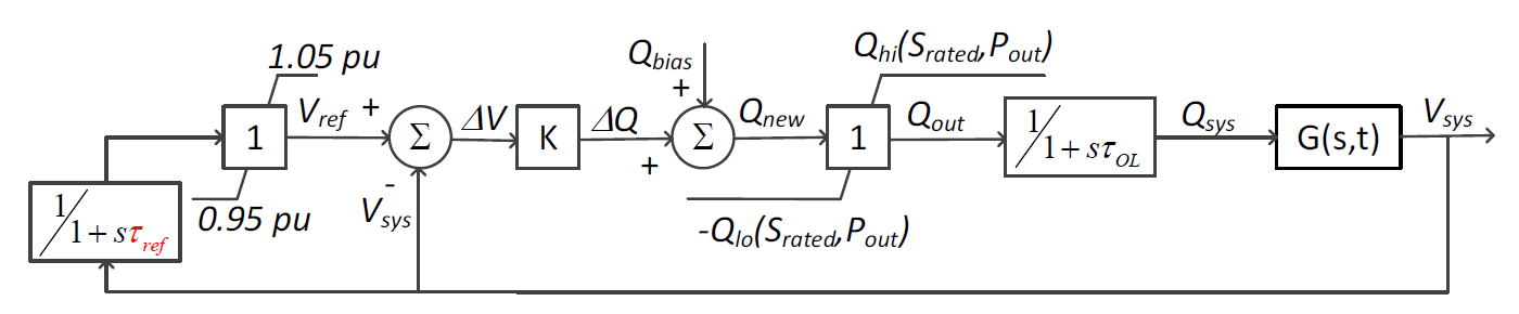
Figure 1: Control block diagram of the autonomously adjusting Vref with time constant τref .

Figure 2: Translating K to the parameters of Figure H.4 of the standard [1], using passive sign convention on Q.
Key Parameters of ExpControl
The ExpControl does not require linkage to a piece-wise linear curve. Its most important parameters are:
• Slope – the gain, K, in Figure 1. The default value of 50 is usually stable, but higher than the maximum allowed value of 22 for Category B inverters [1].
• VregTau – the time constant, τref, in Figure 1. The default value of 300s is recommended.
• DeltaQ_factor – still under investigation; this reactive power “acceleration factor” may need to be specified at 0.2 to 0.3.
• Tresponse – with reference to Figure 1, this is the time for the change in Qsys to reach 90% of the commanded change in Qout. Defaults to 0 for backward compatibility, but should otherwise be set to 10s for Category A inverters or 5s for Category B inverters. Tresponse = 2.3 τOL. (The
InvControl LPFtau attribute is similar, but defined for 95% response instead of 90% response.)
• PreferQ – if required, curtail P to meet the commanded Qout. Defaults to false for backward compatibility, but new models should specify true, as required in [1].
• Qbias – an optional steady‐state dispatch of reactive power, indicated in Figure 1. In per‐unit of each controlled PVSystem kva rating. Negative to absorb Q, positive to inject Q. Defaults to 0. If linked to an external reactive power dispatcher, this would be the signal input connection.
The following parameters are less commonly specified:
• Vreg – initial Vref in per‐unit of the PVSystem’s voltage rating; this is less important because it will dynamically adjust to each PVSystem’s terminal voltage early in the simulation.
• VregMin – leave at the default 0.95 pu
• VregMax – leave at the default 1.05 pu
• QmaxLag – prefer use of PVSystem kvarLimit, unless the absorption and injection capabilities are different.
• QmaxLead – prefer use of PVSystem kvarLimit, unless the absorption and injection capabilities are different.
• PVSystemList – usually left blank to control all PVSystem components in the model
• Basefreq – as with other OpenDSS components
• Enabled – as with other OpenDSS components
• Like – as with other OpenDSS components
• EventLog – used to debug control actions in the case of non‐convergence
The circle‐diagram limits on Q, as depicted in Figure H.2 of [1], have not yet been implemented. The ExpControl was initially developed before [1], and it keeps the name Vreg in place of Vref
Examples from 2019 PVSC
The test circuit in Figure 3 was analyzed in [2] and distributed with OpenDSS under the sub‐directory Examples/ExpControl. You can run the following example by pasting lines 1‐26 into an OpenDSS script window. Note that line 3 should be modified to match the example installation directory on your own computer, so that OpenDSS can find the included Hours.csv, VshapeHi_dss.csv and pcloud.csv.
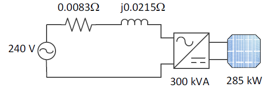
Figure 3: Single‐phase test circuit representing one phase of a utility‐scale PV about 15 miles from the substation
Clear
New Circuit.CloudAdap
cd c:\opendss\distrib\examples\expcontrol
New Loadshape.Vshape npts=1441 interval=0
~ hour=(file=Hours.csv) mult=(file=VshapeHi_dss.csv)
New Loadshape.Cloud npts=86401 sinterval=1
~ csvfile=pcloud.csv action=normalize
New Vsource.Vth1 bus1=2a basekv=.240 R1=0.0083 X1=0.0215 phases=1
~ daily=Vshape
New line.line1 bus1=2a bus2=3a switch=yes phases=1
New PVSystem.PV1 bus1=3a phases=1 kV=.240 irradiance=1 pmpp=285 kVA=300
~ daily=Cloud %cutin=0.1 %cutout=0.1 varfollowinverter=true kvarlimit=132
new monitor.pv1v element=line.line1 terminal=2 mode=96
new monitor.pv1pq element=PVSystem.PV1 terminal=1 mode=65 PPolar=NO
new monitor.pv1st element=PVSystem.PV1 terminal=1 mode=3
set controlmode=static
set maxcontroliter=1000
set voltagebases=[.415692]
CalcV
New ExpControl.pv1 deltaQ_factor=0.3
~ vreg=1.0 slope=22 vregtau=300 Tresponse=5 // EventLog=Yes
solve mode=daily number=86400 stepsize=1s
plot type=monitor obj=pv1pq channels=[1,2] bases=[300,300]
plot type=monitor obj=pv1st channels=[5]
plot type=monitor obj=pv1v channels=[1] bases=[240]
Lines 4‐5 and 7‐8 implement a grid voltage that varies even in the absence of solar power fluctuations. The case can be repeated with unity power factor, by commenting out lines 20‐21. Figure 4 plots the PVSystem output and some voltages of interest. To the right, Vref starts at 1 per‐unit, and quickly adapts to the grid voltage, Vsys or Vunity, which is about 1.03 per‐unit. The reactive power, Q, is zero during the initial adaptation of Vref because there is no real power output, P, during this time, coupled with varfollowinverter=true in line 12. From about 1030 through 1600 hours, P fluctuates and this causes voltage fluctuation. At unity power factor, the Vunity fluctuations are about 3%. The Vsys fluctuations are mitigated to about 1% by the ExpControl, with approximately zero net Q integrated over the day. The Vref signal follows and smooths the Vsys fluctuations by using ExpControl.
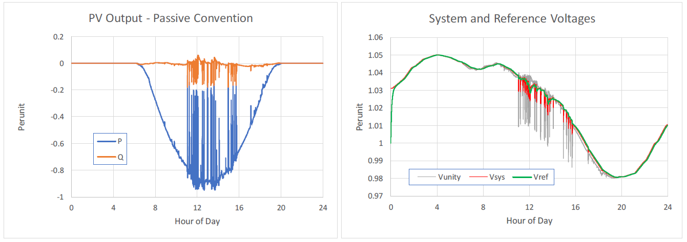
Figure 4: ExpControl produces near‐zero net reactive power over time (left), while suppressing voltage fluctuations around the
system voltage (right).
At around 2000 hours, P cuts out, but the value of Q is already close to zero because Vsys is close to Vref. In other cases, the sudden cut‐out of Q may lead to a significant voltage step. This might be mitigated with varfollowinverter=false, or by ramping Q, which is not currently required in [1]. For convenience, batch‐mode simulation and plotting scripts have been provided:
• Run Master.dss to create results for a clear day with AVR and zero average Q, a cloudy day with
AVR and absorbing ‐90 kVAR average Q, and a cloudy day at unity power factor.
• python plotadapq.py to visualize the effect of absorbing ‐90 kVAR average Q
• python plotadaptive.py to visualize the effect of AVR on clear and cloudy days
• python plotunity.py to visualize the effect of AVR vs. unity power factor on a cloudy day, producing Figure 4.
Comparison to InvControl and CA Rule 21 Smart Inverters
In California’s Rule 21, phase 1 smart inverters have a function comparable to InvControl mode=VOLTVAR, while phase 3 smart inverters have a function comparable to InvControl mode=DYNAMICREACCURR [3]. These are denoted VV and DRC, respectively. The VV mode gives preference to real power, while the DRC mode may give preference to either real or reactive power. The DRC mode may be used either in conjunction with VV, or exclusively. One difference between DRC and ExpControl is that DRC uses a windowed moving average, while ExpControl uses the exponential time
delay. The VV mode in InvControl also has the option for a windowed moving average on Vref, but this option was not adopted in CA Rule 21.
Of the CA Rule 21 options, “Dynamic Reactive Current Support Mode” in phase 3 is the closest to ExpControl. It should give preference to reactive power, and should not be combined with phase 1’s “Dynamic Volt/Var Operations”.
Of the InvControl options, uncombined DRC is the closest to ExpControl.
Use with Storage Elements
As is the case with InvControl, the ExpControl cannot be used with Storage, only with PVSystem. However, the voltage control capabilities it represents from [1] would apply equally well to storage systems. In a future version, both InvControl and ExpControl may be linked to Storage in OpenDSS. In the
meantime, the following workaround can be used to implement reactive power control of storage systems:
• Add a parallel PVSystem with negligible real power (Pmpp), but kva rating equal to the storage system’s reactive power rating, leaving kvarLimit unspecified. Let VarFollowInverter default to False, so the inverter can supply rated Q throughout the day.
• Attach ExpControl to the fictitious PVSystem to implement voltage/reactive power control on the storage system.
The same workaround applies to InvControl. A sample input listing fragment follows; it’s part of a larger model in which a small impedance separates the bess1 bus from the pcc1 bus.
new Storage.bess1 bus1=bess1 phases=3 kV=13.2 kWrated=6000
~ kva=7000 kWhrated=48000 kWhstored=24000 dispmode=follow daily=cycle
New PVSystem.bess1 bus1=pcc1 phases=3 kV=13.2 irradiance=0.5 pmpp=1
~ kva=3600 varfollowinverter=false
New ExpControl.bess1 pvsystemlist=(bess1) deltaQ_factor=0.3
~ vreg=1.0 slope=22 vregtau=300 Tresponse=5
Examples from 2023 General Meeting
A revised application guide for IEEE 1547 [4] is now in ballot resolution, containing new material on voltage response in clause 5. This revision to IEEE 1547.2 should be published in 2023. To provide additional background on the autonomously varying reference voltage, a conference paper has also been submitted for the IEEE PES General Meeting [5]. Examples from the conference paper are now distributed with OpenDSS:
• NantucketExpSteps.py creates Figure 4 of the paper, using the OpenDSS COM interface. The network model is embedded in the Python source.
• Nantucket.xlsx contains data and formulas that created Table I of the paper.
• Hawaii.py creates Figure 5 of the paper, using the OpenDSS COM interface. The network model is embedded in the Python source.
• SCErun.py simulates the secondary circuit example; use command line argument no to run without AVR and yes to run with AVR. The network model is embedded in the Python source.
• SCEplot.py creates Figures 7‐8 of the paper, from the results of SCErun.py. Use command line arguments no and yes.
These examples were tested with OpenDSS v9.5.1.1 and OpenDSSCmd v1.7.6.
Figure 5 simulates the 18‐DER SCE was with 5 times and 10 times the default gain, or K=110 and 220, respectively. The DeltaQ_Factor must be reduced from 0.3, to 0.06 and 0.03, respectively, for the simulations to converge. The OpenDSS simulations take longer than for K=22, but the result is stable. The total real energies remain at ‐6483.62 kwh, but the total reactive energies increase to 135.35 and 316.52 kvarh.
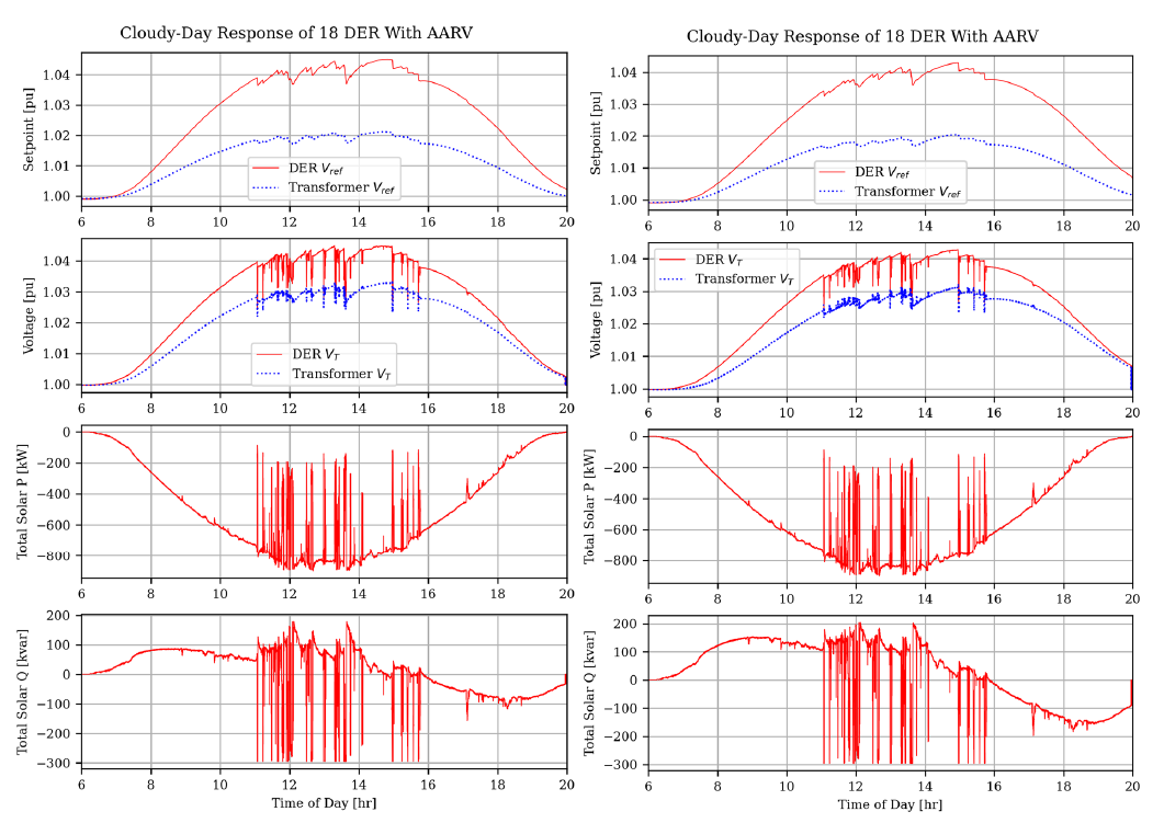
Figure 5: SCE case with K=110 (left) and K=220 (right)
References
[1] IEEE, "IEEE Standard for Interconnection and Interoperability of Distributed Energy Resources with Associated Electric Power Systems Interfaces," IEEE Std 1547‐2018 (Revision of IEEE Std 1547‐2003), pp. 1‐138, 2018.
[2] T. E. McDermott and S. R. Abate, "Adaptive Voltage Regulation for Solar Power Inverters on Distribution Systems," presented at the IEEE Photovoltaic Specialists Conference (PVSC‐46), Chicago, 2019. [Online]. Available: https://doi.org/10.1109/PVSC40753.2019.8981277.
[3] California Energy Commission. "Rule 21 Smart Inverter Working Group Technical Reference Materials." https://www.energy.ca.gov/ electricity_analysis/rule21/ (accessed 2019).
[4] "IEEE Application Guide for IEEE Std 1547(TM), IEEE Standard for Interconnecting Distributed Resources with Electric Power Systems," IEEE Std 1547.2‐2008, pp. 1‐217, 2009, doi: 10.1109/IEEESTD.2008.4816078.
[5] T. E. McDermott, "Autonomous Voltage Response for Distributed Energy Resources [submitted]," presented at the IEEE PES General Meeting, Orlando, FL, July 16‐20, 2023.