The general procedure for the fault study mode (mode=FAULTSTUDY) is described in the previous topic. The mathematics that supports this are described here.

OpenDSS builds a nodal admittance (Y matrix) model of the system. This can be represented schematically as shown in Figure 1. Voltage sources are converted to Norton equivalents and the resulting admittance is incorporated into the system Y matrix as being connected to ground. This includes the Vsource objects and any Generator objects after they has been converted to a dynamic equivalent.

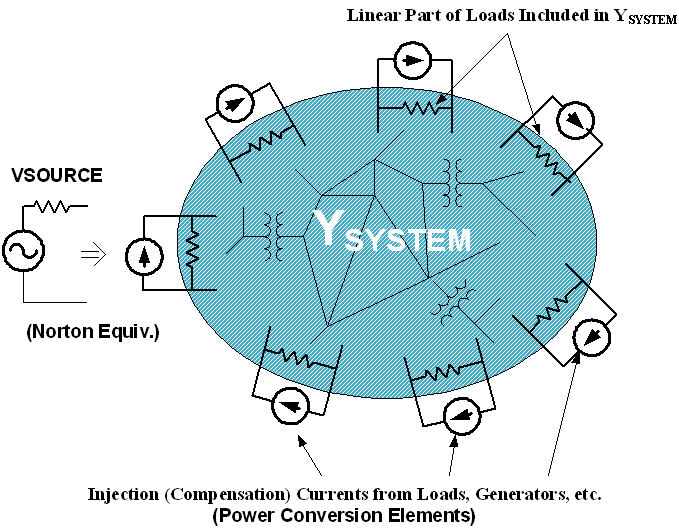
Figure 1

I=YV

I is the vector of injection currents from the current sources shown.  V isthe vector of node voltages with respect to the "ground" reference.

As indicated, OpenDSS then solves the equation I=YV for the voltages to ground. The "I" vector is the vector of current injections into the network. In the usual case, this includes the source currents shown as well as the portion of the load currents not included in the Y matrix already.

The fault study is based on a multiphase Thevinen equivalent at each bus (Figure 2). The first step is to compute the open circuit voltage vector, Voe, at each bus. This is done by performing a direct solution immediately after entering the FAULTSTUDY mode. Keep in mind the solution was previously solved in a standard SNAPSHOT mode, which is not necessarily direct mode.. That serves to initialize the generator models (and anything else that might need it). Then the short-circuit impedance matrix, Zsc, is computed for each bus and inverted to form Ysc. Both forms are retained by the program internally for each bus because there are several useful things they can be used for.

The Norton form of the equations is also retained by computing the short circuit current vector, Isc, that corresponds to the open circuit voltages.

Figure 2. A Multiphase Thevinen (Short Circuit) Equivalent

Since, the system Y matrix already assumes that the voltage sources are shorted, Zsc is determined by injecting a current of 1.0 +j0.0 amps into each node of the bus under consideration -- one node at a time. The resulting voltage vector represents one column of Zsc (See Figure 3).

Figure 3. The voltages are one column of Zsc

This process is repeated for each node at the bus, including neutral nodes or other non-phase nodes. When this is complete, Zsc is fully populated. It is then inverted to form Ysc. Note, there are circuit conditions where Zsc might be a little bit ill-conditioned. In order to inject 1+j0 into a node, there must be a return path. It is possible to set up a condition where this path does not exist, although OpenDSS takes steps to minimize this occurrence. Transformers are the main culprit, but a user could conceivably create a coupled inductance matrix with a line or reactor and leave both ends hanging. OpenDSS adds a tiny conductance to each winding to prevent this, but can't catch everything. This is just a fact of life when doing nodal admittance models and is also encountered in other programs such as EMTP, EMTDC, and SuperHarm. (OpenDSS traps this automatically and is thus more user friendly than any of these in this regard.)

 Ysc = Zsc-1

Figure 4

The Norton currents (short-circuit currents) are now computed as shown in Figure 5. This is the "all­ phase" fault current that the DSS reports. That is, it is the short circuit currents that will flow from each node if all nodes at the bus were shorted to Node 0. Note that these currents will not be equal if the impedances are not balanced (or the open circuit voltages not balanced).

Isc = Ysc Voc

Figure 5

The quantities reported for single-phase faults (each node-to-ground, one at a time) are computed as shown in Figure 6 for a typical three-phase case. The current is computed from Zsc in a straight forward manner because there is no current flowing from the other nodes at the bus. The unfaulted phase voltages are also of interest and are computed as shown from Voe and the computed fault current. If the base voltage is defined for the bus, OpenDSS reports the voltages in per unit. Otherwise, they are in L-N actual volts.

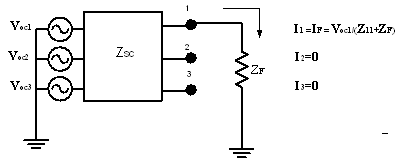
Figure 6

The phase-to-phase faults are a little tricky in one sense, but simpler in another. The Norton equivalent at the bus is employed rather than the Thevinen. Figure 7 shows the equations.

Figure 7

Isc = [Ysc + YF] V

A fault admittance, YF, is connected between the two phases of interest. It is added to the Ysc matrix in the appropriate terms. (Add YF to the two diagonals involved and -YF to the off-diagonals between the two nodes.) Very simple to code. Then, given Isc, the voltages, V, at the nodes are computed by solving the linear equations. Thus, there is no need for further calculations to determine the voltages appearing at the nodes. The fault current in this specific case for a fault from node 1 to node 2 is then computed as:

IF=YF(V1-V2)

OpenDSS initially reported only adjacent phase faults (1-2, 2-3, 3-4, etc.), but now reports all combinations of phase-phase fault currents. For buses that have many nodes, this can be a very large report! Of course, a program using the OpenDSS COM interface can extract Zsc and do whatever it pleases.