OpenDSS Documentation

This document describes how the Dynamics mode solution in the OpenDSS program works. Examples are provided from the Generator element, which is currently the most common element used in simulations in Dynamincs mode.

The Basic Algorithm

Each time step in the dynamics mode solution executes the following steps (extracted directly from the code in SolutionAlgs.Pas):

Increment_time;

{Predictor}

IterationFlag := 0;

IntegratePCStates;

SolveSnap;

{Corrector}

IterationFlag := 1;

IntegratePCStates;

SolveSnap;

The algorithm is currently a simple predictor-corrector method with one step of correction. The IterationFlag variable indicates to the integration routines whether the solution is in the predictor step or the corrector step.

The dynamics algorithm was first implemented with no corrector step, but after some experimentation it was found that the machine electromechanical transients behaved much better with one step of correction.

The IntegratePCStates function cycles through each Power Conversion (PC) element in the circuit and executes its IntegrateStates function. IntegrateStates is a virtual function that is overridden in models that actually have something to integrate. For example, Generator elements have state variables to integrate. However, others do not and this function is simply empty.

Only PC elements have states that are integrated. Power Delivery (PD) elements are constant impedance elements simply defined by a primitive Y matrix.

Going into Dynamics Mode

The first requirement is to get a solution to the base power flow to initialize the dynamics solution. This is to initialize the state variables of the various dynamic elements to approximately match the power flow. If the power flow will not converge, you can do a "direct" solution, which is a non-iterative solution with PC elements (Loads, etc) modeled as constant impedances. This is generally good enough to initialize the voltages at the generator terminals.

In addition to Dynamics mode, the OpenDSS program goes into dynamics solution mode for FaultStudy and MonteFault (MF) solution modes so that contributions from Generator objects and other active objects are more accurately captured.

The steps the program executes when going into Dynamics mode from one of the power flow solution modes is as follows:

• Initialize state variables in all PC Elements

- For example, in a Generator object currently:

▪ Compute voltage, E1, behind Xd' to match power flow (approximately)

▪ Initialize the phase angle, θ, (power angle) of equivalent voltage source

• Set derivatives of the state variables to zero

- For the Generator,

▪ Speed (relative to synch frequency)

▪ Angle

• Set controlmode=time

- When running in time steps of a few seconds or less, controls that depend on the control queue for instructions on delayed actions will be automatically sequenced when the solution time reaches the designated time for an action to occur.

• Set a flag to preserve Node voltages in case Y matrix changes.

- Y matrix changes could occur if a switch were to open during the simulation, which might re-order the bus lists. This flag prevents loss of data by reassigning the Node voltage after the re-ordering.

Integrating the State Variables

Integration is performed within the PC element modules themselves, not in the Solution module. Therefore, it is possible to have different integration formulae for different classes of devices.

As of this writing, the Generator employs a simple trapezoidal-rule predictor-corrector integration method. This will be described in the next section.

Predictor and Corrector Steps

The predictor step offers algorithm designers the opportunity to insert a predictor formula at the beginning of the process. It may differ from the corrector step only in that it updates the initial value of the state variables for this time step based on derivatives at previous solution. The following three steps are performed for both the predictor and corrector steps:

1. Compute derivatives for this time step

2. Integrate state variables

3. Solve the circuit with this guess

For the present implementation of the Generator object, the state variables are the speed (relative to synchronous speed) and the shaft angle, θ . The derivatives of these are computed and then integrated in a trapezoidal formula as follows:

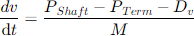
Where: 

v = shaft speed (velocity) relative to synchronous speed

θ = shaft, or power, angle (relative to synchronous reference frame)

Pshaft = shaft power

Pterm = terminal power out

D = damping constant

M = mass

Integration

Trapezoidal integration formula for θ, for example:

Δt= time step size

In the Predictor step, the integration routine captures the state variables and their derivatives from the previous time step (moves the (n+1) values to the n values in the formulae above). Then it makes a Predictor calculation of the derivatives at the new step based on the present values of the state variables.

Based on the results of the Predictor step, a new guess at the derivatives at the present (n+1) step is computed in the Corrector step. Then the guess at the state variables is corrected.

Only one Corrector step is executed. A circuit solution is performed between the predictor and corrector steps and after the corrector step.

Circuit Solution in Dynamics Mode

The circuit solution proceeds more or less like it would for a normal power flow solution. The Load elements are presently treated the same since load dynamics have not been implemented. They are sinks or sources of power, depending on sign. However, the Generator, and any other elements with dynamics models, will behave differently. The present implementation of the Generator model computes its terminal currents using the voltage source, adjusted for the new phase angle computed by the integration steps, rather than a specified power and power factor as it is modeled in a power flow solution. Thus, the power from the Generator will depend on system conditions with might be the result of a disturbance (that’s usually why you would be simulating dynamics).

As a point of reference, in Harmonics mode, the Loadmodel option is set to Admittance and a direct solution is performed. This is a non-iterative solution mode. However, in Dynamics mode, the load flow is normally solved iteratively for each guess at the Generator voltages.

Computing Terminal Currents in Dynamics Mode (Generator)

As an example of computing terminal currents, we will examine the default Generator object algorithm since it is the most commonly used at present. The electrical model for a 3-phase Generator object is illustrated in Figure 1.

Figure 1. Default Model of Electrical Part of Generator Object in Dynamics Mode

In any of the power flow modes (Snapshot, etc), the Generator object is treated as a power source like most other power conversion elements. Upon entering dynamics mode, the Generator is converted to a positive-sequence voltage source behind a reactance of the form shown in Figure 1. Note that this is a symmetrical component model with the generator part being represented by positive- and negative-sequence networks as shown.

The positive-sequence network consists of a voltage source, E1 ∠ θ, behind the value specified for the Xdp property of the Generator model, representing the transient reactance, Xd’. E1 and θ are initialized so that the initial solution in dynamics mode approximates the most recent power flow solution. Thus, simulations will be better if the initializing power flow solution is reasonably well balanced (i.e., no fault conditions – do that after entering dynamics mode). The generator excitation is assumed to be only positive sequence.

The negative-sequence network consists of the value specified for the Xdpp property of the Generator. This is usually closer to the actual negative sequence reactance of a machine. The actual negative sequence reactance of the generator many be entered for Xdpp if known.

The terminal currents are computed as follows:

• The phase domain (ABC) voltages are transformed to symmetrical component (012) voltages.

• The symmetrical component currents are computed based on the present value of E1 and θ.

- θ is determined in the integration step. In the default model this is based on a simple single-mass model and the difference between the shaft power and the electrical power.

- In the default model, no exciter or governor action is modeled. Therefore, E1 and the shaft power remain constant for the duration of the simulation. User-written modules could change these values.

• Finally, the symmetrical component currents are transformed back into the phase domain. The terminal currents are used to compute the compensation currents that are used in the circuit solution algorithm (see below).

Compensation Currents

Once the terminal currents have been computed, the compensation currents from all PC elements that appear in the system nodal admittance equations in the Normal solution mode are computed (see Figure 2).

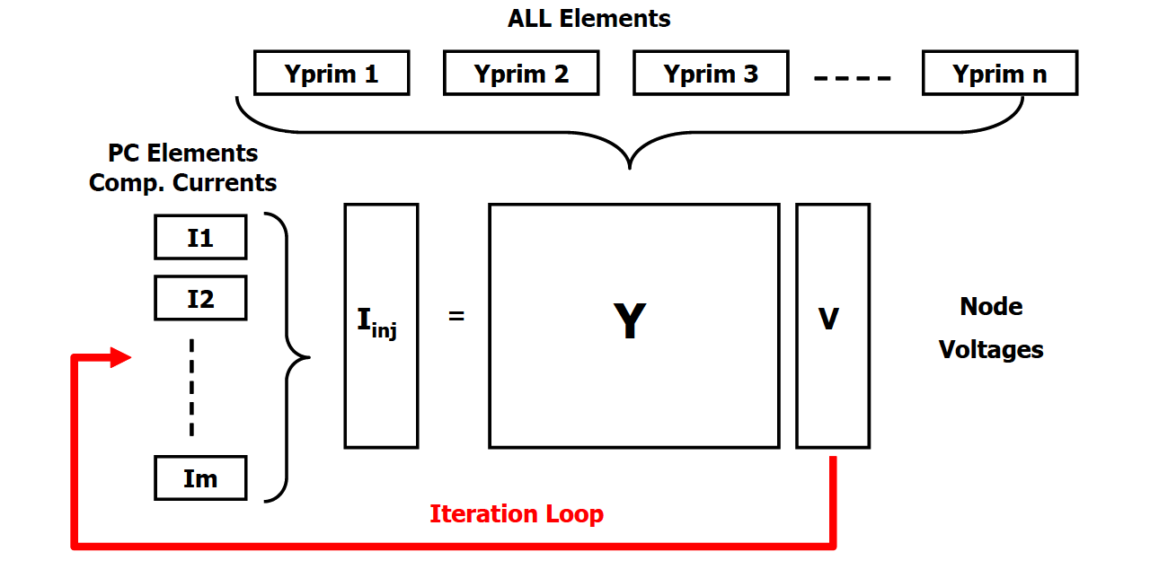
Figure 2. Normal Solution Iteration Loop

These currents are the values of the current source in the Norton equivalent representing the Generator. This is illustrated in Figure 3. The equivalent consists of a constant impedance (actually, admittance) part that is included in the system Y matrix in Figure 2.

Figure 3. Norton Equivalent Model of Power Conversion (PC) Elements

For the default Generator model, the constant impedance part of the model represented by the Yprim matrix would yield the power at the time of entering Dynamics mode if the terminal voltage were 100% of the specified rated voltage. The compensation current is the difference between the terminal currents computed as described above and the currents in the Yprim branch.

Each element of the multiphase compensation current array is added into a particular element of the Iinj array shown in Figure 2. The Iinj array is a collection of the Norton equivalent current sources in all the PC elements in the circuit.

Computing Terminal Currents in Dynamics Mode (IBRs)

Modeling Inverter-based generation resources (IBRs) such as solar PV and energy storage in the frequency domain requires a simplification given the digital control signals, they require for operating. In this case we have adopted the simplification proposed by Yazdani [1]. This simplification proposes a simplified model plus an average control signal for emulating the PWM control signal in the frequency domain. This model considers the electrical model for the half-bridge inverter shown in Figure 4.

As can be seen in Figure 4, the inverter model represents the DC voltage sources feeding the inverter bridge, as well as the RL series filter for interfacing the dc and ac sides of the inverter. The gates of the IGBTs are controlled by a digital control signal, normally driven by a PWM modulation. For the proposed model it is averaged using a modulating signal that represents the duty cycle of the PWM control signal as shown in Figure 4 and Figure 5.

7

Figure 4. Half bridge inverter schematic plus RL series filter [1].

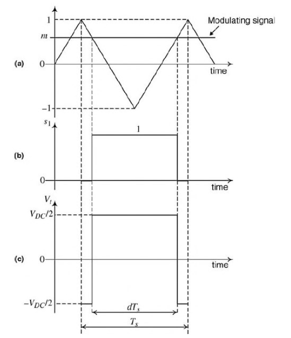
Figure 5. Averaged control signal for emulating PWM duty cycle [1]

This model is compatible with other dynamics included in OpenDSS based on differential algebraic equations. This modeling approach facilitates the inclusion of the inverter dynamics into OpenDSS, facilitating its adoption and compatibility with the existing dynamic-oriented objects such as dynamics expressions object, DynamicExp (presented in previous reports). The equations describing the inverter’s dynamic behavior based on Figure 4 is as follows:

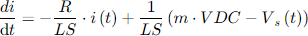
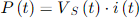
Where m is the modulating control signal, VDC is VDC/2 in Figure 4, Vs(t) is the magnitude of the ac voltage at the inverter ac side, R and L are the resistance and inductance in Ohms and mH, respectively, for the series RL filter. The output power, P, is calculated considering the voltage at the inverter ac side.

R and L are calculated internally by OpenDSS considering the DER ratings as follows:

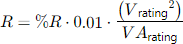
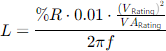
Where %R and %X are the percentage of R and L assigned to the DER when declared in OpenDSS. If the user prefers to use his own values for R and L, it is possible by using Dynamic expressions (see at the user manual Dynamic expressions).

The digital controller for the inverter is implemented using a proportional-integral (PI) controller that can be configured through OpenDSS commands using a proportional gain. The controller is used for calculating the modulating signal value (m) at each simulation step as shown in Figure 6.

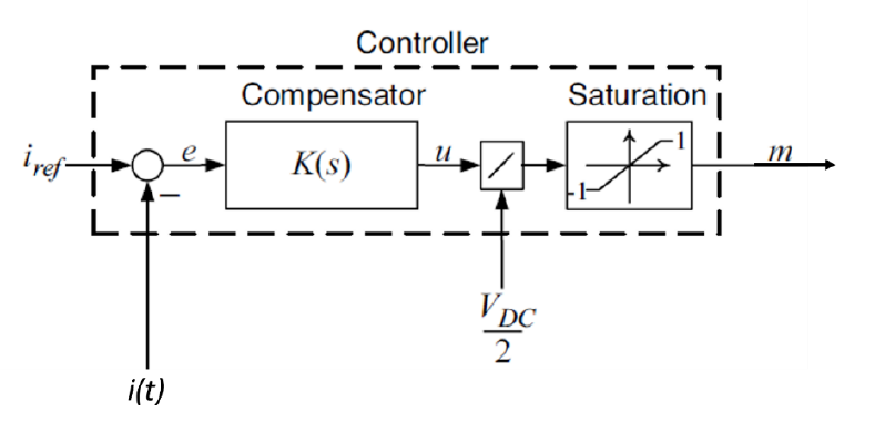
Figure 6. PI controller implemented for controlling the inverter’s duty cycle [1]

The commands needed for configuring the dynamics features of inverted-based DER such as solar PV and energy storage in OpenDSS are described in Table 1. These commands allow users to characterize inverters accurately, allowing the controller to move into underdamped, critically damped, and overdamped regions for describing the inverter’s dynamics. 

Table 1 OpenDSS controller properties for configuring dynamics of inverter-based DER

Dynamics behavior in time for PV system

The PV system power output is governed by several variables including the irradiance and, efficiency of the panel, among other parameters The irradiance is the most critical for determining the panel’s power output during operation. This power output is followed in dynamics simulation for recreating the dynamic behavior of the inverter considering the actual irradiance, efficiency, temperature, and other variables that affect the power generation for the panel array.

This condition requires the user to consider the hour of the day if an irradiance profile is linked to the PV system characterization. It is also recommended to enable the load shape class for which the irradiance/temperature profiles are associated to the PV system in case these must be reflected in the dynamics simulation. An example of this condition is illustrated in Figure 7. The code used in OpenDSS for generating the output seen in Figure 7 is as follows:

…

New "PVSystem.mypv" phases=3 conn=delta bus1=PVBus daily=pvshape kv=0.48 kVA=2000 Pmpp=2000 kVDC=0.6 %R=50 %X=50 Kp=0.006 PITol=1 SafeVoltage=0.01

Solve

Set mode=dynamics time=(12,0) stepsize=0.0001 number=5000

Solve

Set time=(12,120)

Solve

Set time=(12,181)

Solve

Figure 7. Power production of PV in dynamics mode considering irradiance

Dynamics behavior in time for Storage devices

Storage devices will also follow the profiles assigned for their control in time. It is important to realize that for the dynamics simulation the storage device will not assume the Discharging state by default, but instead, it needs to be specified by the user.

Safe mode

Safe mode is a feature that turns OFF the inverter if the ac voltage at the output of the inverter is below a certain value, representing a risk for the inverter integrity. In the case of PV systems, the PV will turn ON again automatically after the voltage at the inverter terminals is within an acceptable value for the inverter operation. While the inverter is in safe mode, the flag SafeMode will be set True, otherwise, it should report False.

On the other hand, when entering in safe mode, the storage device will turn the inverter OFF and set itself into IDLING mode. Once the voltage at the inverter terminals in the safe region the storage will not go back to DISCHARGING automatically, requiring intervention by the user or the control software driving the simulation.

Model performance

For evaluating the performance of the newly added dynamic model for inverter-based DER, a large-scale circuit model was proposed for incorporating multiple generators and evaluating their response when exposed to faults on the distribution feeder. This will be important for successfully integrating wind generators with other DER that might be present on a feeder in the future.

The circuit model is the IEEE 8500-Node Test Feeder. This was modified for hosting three induction machines representing wind generators, one PV system and Storage device for voltage support. All connected to the grid through transformers and the ac-side interconnection modeled in the delta configuration. In OpenDSS, invert-based devices are typically modeled in delta configuration because they are not connected to the system neutral. A delta configuration limits the current contribution to the positive- and negative-sequence currents. The model features are presented in Table 2. The model implementation for this test is shown in Figure 8.

Table 2 Technical features for IEEE8500 nodes test case.

Figure 8. IEEE 8500 nodes test system used for dynamics simulation

In this example, there are three wind generators, 1.5 MVA each, 3 phase. We have also added a large solar generation plant of 2 MW. In this case, the power output is entirely active power as is typical for most PV systems (DC/AC ratio = 1). This PV system follows the irradiance profile shown in Figure 7. Next to it, there is also a storage device rated 2 MW, 4MWh for power support as shown in Figure 8.

To visualize the dynamics response of the DER deployed across the model the following conditions are forced:

1. A 3-phase line-to-ground fault will be added at two different points of the model.

2. The Safe Voltage level for the inverter-based resources (PV and Storage) has been lowered to 1% to let the inverters try to “catch up” with the fault.

3. To match with previous reports, the fault is cleared after 70ms.

4. The simulation time step for this simulation is 0.1ms. The time of the day is 12PM for allowing the PV system to generate above the 80% of its rated capacity.

The dynamic features for both, the PV and storage models in OpenDSS, are as follows:

Table 3 Inverter-based DER dynamics features

Case 1

The fault is inserted at bus m1142828, close to the PV and storage downstream on one of the feeder branches as shown in Figure 9.

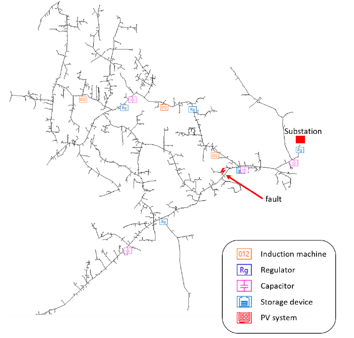
Figure 9. Applying fault at bus m1142828

After recovering the model from the fault, the PV and storage inverters try to catch up with the voltage sag introduced by the fault, the control signals for the PV and storage inverters are as shown in Figure 10a and Figure 10b respectively.

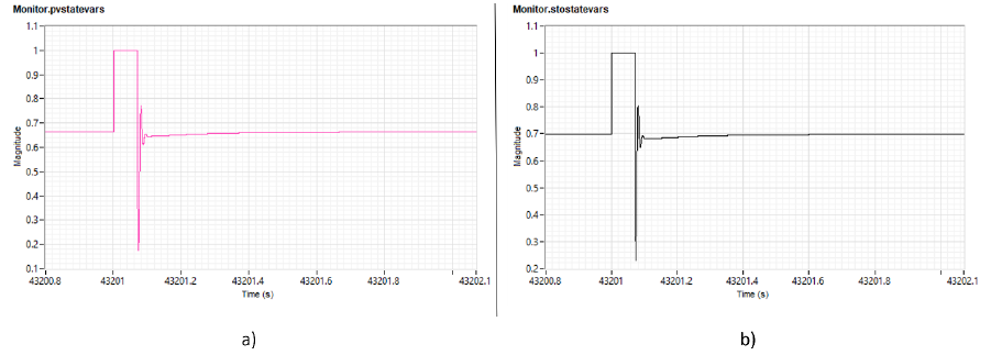
Figure 10. Averaged modulation signal for a) PV panel array and b) Storage device

These modulations signals reveal that the storage device is the one prevailing while trying to regulate voltage, reaching saturation given the severity of the voltage sag. On the other hand, the PV follows the storage device effort by compensating using the voltage at the point of connection as reference, reaching saturation as well. The power delivered by both devices is shown at Figure 11.

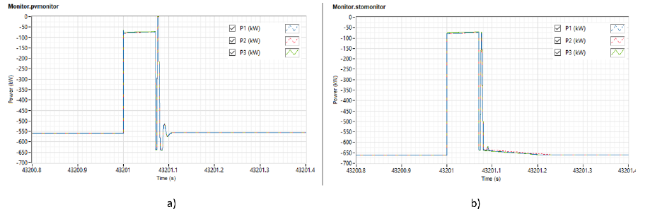
Figure 11. Power output for a) PV system and b) storage device

The generators respond accordingly and get back to their normal operation after a few oscillations dictated by their damping constants as shown in Figure 12.

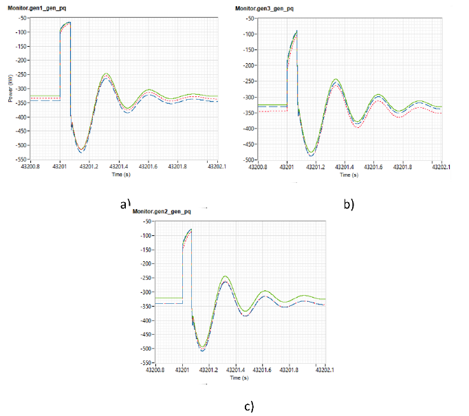
Figure 12. Power output for ) generator 1 b) generator 2 and c) generator 3

Case 2

The fault is inserted at bus m1069496, at 3.077 mi from the PV and storage and between the generators as shown in Figure 13.

Figure 13. Case 2, fault inserted at 3.077 mi from PV and storage

Because the voltage sag is not as severe as in Case 1, the inverter controllers for PV and storage don’t reach saturation as shown in Figure 14. Despite not reaching saturation at control level, the saturation is reached due to the hardware level not being able to deliver the target current (amps). The power delivered by these devices in not enough for maintaining the system within the voltage range before the fault is cleared. The currents generated by the PV and storage are shown in Figure 15.

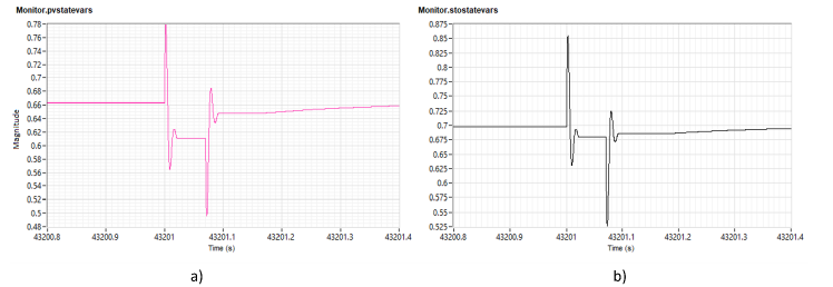
Figure 14. Averaged modulating signal for a) PV system and b) Storage device (Case 2)

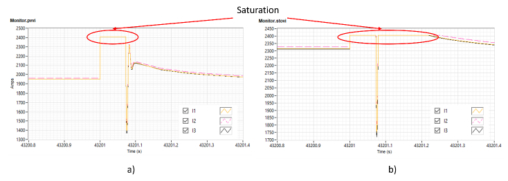
Figure 15. Output currents for a) PV system and b) Storage. Both reach hardware saturation during fault

More examples can be found at:

https://sourceforge.net/p/electricdss/code/HEAD/tree/trunk/Version8/Distrib/Examples/IBRDynamics_Cases/GFL_IEEE123/.

Black Start and Grid Forming Inverter

When forming in Grid Forming inverter control mode (GFM), an IBR provides the services traditionally provided by synchronous generators. For this, GFM inverters differ from the operational features of Grid Following (GFL) inverters in several areas. One aspect is that GFL affords the opportunity to energize a section of the grid (which would have been typically provided by a GFM inverter) and it can also coexist and facilitate energy transactions with other GFL inverters within the same circuit.

There are 2 examples provided with OpenDSS for illustrating this concept, these are located at:

https://sourceforge.net/p/electricdss/code/HEAD/tree/trunk/Version8/Distrib/Examples/IBRDynamics_Cases/GFM_IEEE123/. 

In these cases, an island is intentionally formed. This island contains a large storage unit and a solar plant. To keep the microgrid operational, the storage device is configured as grid forming inverter. After setting up the dynamics simulation the storage device starts the restoration process as shown in.

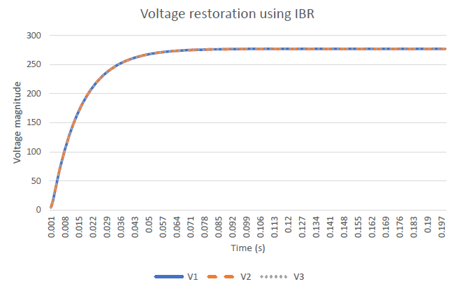
Figure 16. Voltage restoration using IBR

Since the PV system is operating in grid following mode, it follows the safe voltage level (default 80% of nominal voltage) to wait before start generating power. Figure 17 illustrates the power output for both, Storage and PV system. It can be seen how the PV system waits until the voltage level at its terminals reaches at least the 80% of the PV nominal voltage for start generating. The PV power output will also affect the Storage device power delivery as can be seen at the top of Figure 17.

The safe voltage level is a customizable parameter that can be modified to provide the tools for representing different IBR dynamics and automations. It is important to remark that when an IBR is operating in GFM mode, the SafeVoltage parameter needs to be set to 0 to provide black start restoration support.

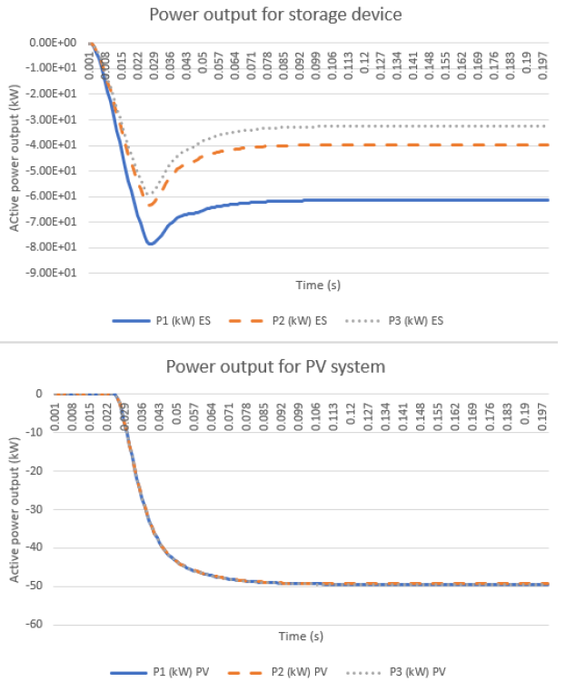
Figure 17. Power output for Energy Storage (top) PV system (bottom)

Sometimes the IBR cannot pick up the load within the microgrid, whereas the actual power output in time such as the case for PV systems is insufficient to energize the load, or because the actual load level surpasses the IBR technical features. In that case, the IBR working in GFM control mode will start the restoration process but after detecting the overcurrent at the IBR’s terminal, it will drive the Inverter to safety by turning it OFF as shown in Figure 18.

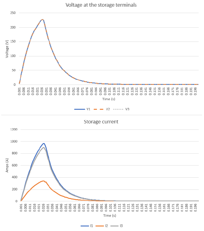
Figure 18. Voltage (top) and Currents (bottom) for storage device when moving to a safety zone

References

[1] A. Yazdani and R. Iravani, Voltage-Sourced Converters in Power Systems: Modeling, Control, and Applications (IEEE Press). Wiley, 2010.