OpenDSS Documentation

State Estimation Background

Most papers on power system state estimation begin with a presentation of a set of equations similar to those shown below

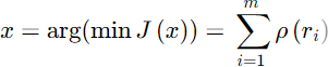
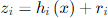
Figure 0-1. Typical statement of State Estimation Equations

This formulation indicates that the objective is to find the set of state variables, x, that results in the minimum error in the measurement residuals, r, based on the function represented by ρ(ri). 

In the classical transmission system power flow estimation formulation, the x vector consists of the voltage magnitude at the buses and the phase angles of the voltages. [1]

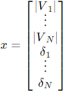
This conforms to the choice of unknown variables in the typical formulation of the so-called Newton- Raphson power flow solution commonly used in transmission power flow programs. The corresponding set of known variables is the mismatch in P and Q at each bus ordered as follows:

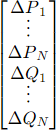
The powers and voltages are related through the admittances of the power delivery network connecting the buses. Then solution process is to use the Newton-Raphson method to drive the power mismatches toward zero.

The classical state estimation method takes a similar approach. It is the measurement error that is to be driven toward zero. This is generally formulated as the difference between the measured and computed powers (complex power, S = P + jQ) at key points in the system. This is represented by the second equation in Figure 0-1. In its most straightforward approach, like the Newton-Raphson power flow, this equation simply involves the admittance matrix, Y, of the linear elements of the power delivery network and the estimates of the voltages, V. This may be expressed mathematically in compact matrix form as

where bold text signifies complex vectors and matrices, T signifies transpose, and * signifies complex conjugate of the terms of the resultant vector. The resultant S vector represent the power injections at each bus.

This scheme yields a system of nonlinear equations that is often solved for x by the Newton-Raphson method, which requires a Jacobian to be formed. In some systems, the Jacobian can be ill-conditioned. If all goes well, and Y is actually a good representation of the lines and transformers in the power system, this system of equations will converge to a reasonable estimate of the voltage magnitudes and phase angles.

Chilard, et. al. [2, 3] have employed the classical method on distribution systems at EDF. Some of the work has been done in cooperation with EPRI. [3] Some success has been reported with this method and an implementation in a DMS is in progress as reported at the CIRED 2011 conference in Frankfurt.

Baran and McDermott [4] point out that this formulation with voltages as the state variables does not always work well for distribution systems. The reasons they stated in their paper were:

• Very few measurements are available, often only voltage and current magnitudes at the substation,

• Switch states and regulator/transformer taps may not be monitored

• Many of the feeder measurements are current magnitude rather than P and Q

• Three-phase unbalances and low X/R complicate the measurement function

Their solution to these problems is to use the branch currents as the state variable, x, instead of the voltages. The advantage claimed for this approach is that the Jacobian can be decoupled by phases and is well conditioned. This is claimed to yield a more robust method for radial feeder applications than the classical voltage-based method.

Roytelman and Landenberger [5] also discuss some of the practical difficulties with distribution state estimation on real distribution systems. They cite:

• Limited observability with only a few measurements available,

• Inconsistent measurements,

• High ratio of current magnitude (|I|), measurements compared to P and Q measurements,

• Lack of measurements on small DG.

For these reasons they assert that distribution state estimation is not as accurate as transmission state estimation, which is presumably a reference to the classical formulation above. They claim this leads to the use of heuristic rules to improve the accuracy. That is, some knowledge and understanding of how the distribution system is expected to operate, and has operated in the past, is employed to improve the estimate. Their approach is to minimize the weighted square error between measurements and estimates of |I|, P, and Q. That is, they include the current magnitude along with the power quantities commonly used in the classical approach.

Impact of Distribution System Design

One explanation for why Chilard, et. al., have apparently had better success with the classical voltagebased method than many of their North American counterparts is that the EDF medium-voltage (MV) distribution systems are more balanced and more like transmission systems. In general, this is true of

most European-style distribution systems (Figure 0-2). In this figure, residential loads are served from the 400 V LV system, which is a conventional 4-wire three-phase multi-grounded neutral system (or a 230 V single-phase system). However, the MV portion, or primary distribution, is typically a three-wire unigrounded system. The MV/LV transformers are connected in delta on the primary side. Single phase units are connected line-to-line. Therefore, no zero-sequence current is present on the MV system.

Figure 0-2. Three-line Schematic of a Typical European Distribution System

In contrast, most North American primary distribution systems are 4-wire multi-grounded neutral systems that contain numerous unbalances. Figure 0-3 depicts some of the key features of this type of system that differ from the European design.

Figure 0-3. Three-line Schematic of Typical North American Distribution System

Residential loads are typically served by the ubiquitous split-phase 120/240 V single-phase transformer. The primary of these transformers are commonly connected line-to-neutral, although there are many line-to-line connected transformers on West Coast systems and on legacy delta systems.

Industrial and commercial loads are frequently served with three-phase transformers. Unlike Europeanstyle systems where the service transformer configuration is more consistently Delta/Wye, one might encounter any of a number of three-phase transformer connections serving the load:

• Grounded Wye/Wye (Yg-Yg): This is generally the most common connection on more recentlybuilt distribution systems (out of concern for ferroresonance on single-phasing incidents),

• Delta/Grounded-Wye

• Ungrounded-Wye / Delta: Common for serving 3-phase loads, particularly motor loads. The primary side neutral is not grounded to prevent providing a “ground source” path.

• Ungrounded-Wye/ Delta w/ center-tapped winding (also called a “4-wire delta”): Common for serving commercial loads with a combination of 120/240 V single-phase loads and 240 V three-phase loads.

• Open-wye/Open-delta: Requires only two phases to serve three-phase loads. Economical way to serve loads such as irrigation pumps that operate only a small fraction of the year or other 3-phase loads in remote areas. In North America, one leg of the delta is frequently center-tapped with the center tap grounded.

• Delta/Delta: Mostly older legacy systems.

• Grounded-Wye/Delta: This connect is prohibited on many systems but is increasingly common as interconnection transformers for DG. Contributes strongly to zero sequence currents.

In addition to loads, there are often numerous capacitor banks on a feeder connected either grounded-wye or ungrounded-wye. Delta-connected banks are found on delta systems and in many industrial power systems. They may be switched or fixed (always on) or seasonally switched. This makes it difficult to estimate the reactive power if their state is not explicitly monitored. In addition, at any given time there are many capacitor banks with fuses blown so that one or two phases are out of service. This can occur simply due to fuse element fatigue after being switched many times or due to excessive harmonic currents, an increasingly common problem.

A few utilities switch each phase of three-phase capacitor banks independently. This has some advantages for controlling the voltage and correcting the power factor when nearly all the load is residential singlephase load connected line-to-neutral. This scheme is employed where residential air conditioning load is prevelant.

In addition to capacitor banks, most feeders have tap-changing transformers for voltage regulators. This can be in the form of substation load-tap-changers (LTC) or line voltage regulators. LTC transformers generally change all three phases in synchronism. In North America, most line voltage regulators and feeder regulators are single-phase autotransformers that are separately controlled. Some regulator banks do have ganged controls so that each phase is on the same tap.

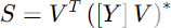
Open-delta regulator banks are used in some rural areas. This is economical because it requires only two regulators to achieve 3-phase voltage regulation on delta systems. However, it is difficult to model. One regulator is in a leading configuration and the other is in a lagging configuration. That is, the tap windings are in opposite polarities. One form of this connection is shown in Figure 0-4. For further reference, the IEEE 37-bus Test Feeder [6] contains an open delta regulator bank.

Figure 0-4. One form of Open Delta Regulator Bank Connection (Source: Cooper R225-10-1)

These characteristics of the North American distribution system significantly complicate the distribution state estimation problem. The discrete positions of tap changers and capacitor switches along with unbalanced transformer and line configurations make it more difficult to boil down the problem into a set of closed form equations that can be easily solved.

Load Models

One issue with distribution state estimation is that the load is less aggregated than at the transmission level. Therefore, it is more important to model its variation with voltage, particularly if there are no P and Q measurements at each load point. The simple power flow model assumes that current and voltage at a load are represented by constant power with P and Q known. The load current for this model varies inversely with voltage magnitude. In most studies of conservation voltage reduction (CVR), P is found to vary somewhat less than linearly with voltage (an exponent of 0.6 – 0.8) while Q varies more than might be expected (an exponent of 3-4). For reference, a constant impedance load would have an exponent of 2: i.e., P and Q vary by the square of the voltage. This can be an important issue because there can be a significant drop in voltage along the feeder. Consider the voltage profiles shown in Figure 0-5 and Figure 0-6.

Figure 0-5. IEEE 8500-Node Test Feeder Voltage Profile at Peak Load

Figure 0-6. IEEE 8500-Node Test Feeder Voltage Profile at 50% Load

There is a 10% voltage difference between the highest voltage along the feeder and the lowest at the peak loading time. The three voltage regulator banks in the feeder also must be properly accounted for. At 50% of peak loading the voltage differences are much less and are clustered toward the high side of the normal band. This characteristic of voltage regulation is quite common.

This example illustrates some of the issues related to estimating the load value and the voltages along the feeder in a realistic distribution feeder with multiple voltage regulating devices. Not only must the load demand be estimated reasonably based on the voltage at the load but the taps on the regulators and the positions of the capacitor switches must be accounted for (six of the capacitors switched off between the 100% peak load case and the 50% peak load case).

Using the OpenDSS for State Estimation

The EPRI OpenDSS program is a distribution system simulator – as its name implies – designed to provide a very flexible platform for system studies and for research into distribution system analysis methods. It is a simulation engine that can be used for multiple purposes and attached to other programs. It was designed to model all the circuit elements and configurations found on the unbalanced North American distribution systems for distribution planning studies. This also gives it more than sufficient capabilities to model the more balanced and regular European style systems.

The OpenDSS originally was built with only a small set of rudimentary circuit solution algorithms. Special algorithms were executed by other programs typically written in MATLAB, Excel VBA, Access VBA, Python, etc. using the interface provided with the OpenDSSEngine in-process COM server. Over

time several algorithms developed in this manner have proven generally useful and have been implemented inside the core of the program for improved execution efficiency. Recognizing that it is impossible to anticipate all the applications users might have for the program, the COM interface was provided to allow users to write their own algorithms outside the program and drive it to achieve specific goals. This is the typical way new algorithms are developed.

With respect to state estimation, there are only a two built-in algorithms at present. Both are related to the common “load allocation” problem that is performed by most distribution system analysis program in one way or another. This is the process of assigning demand values to the numerous load points on the circuit when only the substation current or powers are known. To perform a more closed-form technique like the classical method described previously, a separate program must be used, such as a MATLAB program. The OpenDSS COM interface would be used to provide the necessary data to execute a particular algorithm. For example, the system Y matrix may be extracted along with the voltage magnitudes and angles. One could construct a separate power flow solution outside the program, using the OpenDSS essentially as a data source and repository.

However, there is a good question why one would want to do this because the OpenDSS contains very good facilities for solving the distribution power flow, adjusting loads, etc. The power of OpenDSS for distribution state estimation comes from its ability to model distribution feeders in great detail with all unbalances and special controls represented. As described previously, there are many discrete controls acting on the circuit that must be accounted for. It is often difficult to represent these in any closed form solution. The main technique is to adjust the load model values to match the demand registered at the head of the feeder and, possibly, at special sensors placed along the line. As the load estimates are adjusted, solutions are performed during which the regulator and capacitor controls automatically adjust themselves. Losses are naturally included in the power flow solution and generally do not have to be estimated separately. A better use of the COM interface is to provide tweaks to the internal algorithm to improve the estimate. For example, after an intial guess at the state one could execute a random search algorithm adjusting loads about a nominal mean and switching capacitors in a reasonable scheme to see if a better match to the measurements can be achieved. This has been done more for power quality issues (e.g., harmonic distortion and voltage sag prediction) than load state estimation, but it illustrates how the OpenDSS was intended to be applied for such applications.

By this simulation-based approach to state estimation, the voltages generally stay in a reasonable range. One of the potential problems with the classical approach is that an ill-conditioned problem will produce voltage estimates that are perhaps 10%, or more, too high or low. This almost never happens with the simulation approach that relies more on the measured branch currents and powers to drive the solution. Normal simulation of tap changer action and capacitor switching will generally keep the voltage within 1- 2% of actual.

This technique proved successful for the most of the more than 60 feeders in the EPRI Green Circuits program. Yearly simulations of loading were performed in this analysis. Therefore, it is important to match the loading at all times of the day. The loads were defined by Loadshape objects based mostly on the overall feeder demand shape, but also in some cases on AMI data for individual loads. Generally, the kW shape was relatively easy to match by allocating the loads at peak demand and thereafter adjusting the kW by a selected shape. The kvar characteristic was more difficult to match. Some load allocation algorithms will simply distribute the kvar mismatch among the loads, which often leads to unusual power factors. The approach used in the OpenDSS was to adjust the capacitor switching to make up the bulk of the kvar mismatch and then fine-tune the power factor assumed for the load. Complicating factors included seasonally-switched fixed capacitor banks, capacitors with blown fuses, and capacitor control modeling issues that improperly sequenced the bank switching. Figure 0-7 shows the match achieved in measured and simulated currents over a years using this approach.

Figure 0-7. Example of Match Achieved Between Measured and Simulated Currents for a Circuit in the EPRI Green

Circuits Project

Load Allocation Algorithm

The load allocation process in distribution system analysis distributes the total feeder load to individual load points by some algorithm. While users may write any allocation algorithm of their choosing in an external program, the default method in OpenDSS is described as follows.

A Load object in OpenDSS is simply a standard Power Conversion (PC) element. One of the unique features of OpenDSS compared to more traditional power system analysis program is that Load is not a property of a Bus object. Rather than a Bus having load, a Load is connected to a Bus (just like any other circuit element). In Computer Science object-oriented terminology, rather than “a Bus has Load”, it is “a Load has a Bus”. This may seem a very subtle concept, but it is actually quite important to the Load Allocation problem. Any number of Load objects can be connected to the same bus. Each can have its own model for variation with voltage magnitude and its own loadshape for variation with time. A Bus may have any combination of 1-, 2-, and 3-phase Load objects connected to it. Each could be adjusted differently in the allocation process.

Some Load object rules are:

• If the Load is defined by either kW/PF, kW/kvar, or kVA/PF combinations it is assumed to be known and is not adjusted by the load allocation algorithm.

• The Load must be defined by either its connected transformer kVA rating or kWh billing over a specified billing period to be eligible for allocation. Such Load elements take up the slack, or residual, during the allocation process.

• If connected kVA, the base kW is determined by kW = AllocationFactor * kVA. The default AllocationFactor is 0.5, but may be changed to force the algorithm to force more load into one area than another.

• If kWh billing, the base kW is determined by kW = kWh/(BillingDays*24) * C. That is, it is the average kW time a factor, C. The C factor defaults to 4 but may be adjust programmatically to force different amounts of load into different areas of the feeder.

• Each Load object has an upstream sensor responsible for setting its allocation factors. On a simple feeder circuit, the upstream sensor will be the energy meter (EnergyMeter object) at the head of the feeder. Additional EnergyMeter objects and special Sensor objects may be added to

the feeder to sectionalize the allocation process into smaller portions of the feeder. Therefore, if additional information such as current magnitude or power is available from a device on the line, it may be used to improve the estimate.

• Loads with AMI meters installed are generally exempt from the allocation process. The AMI P, Q data are loaded into a Loadshape object and assigned to a Load object in actual values. This defines the kW and kvar properties of a load or group of loads.

With these elements in place, the load allocation algorithm is straightforward:

1. Solve, computing the load kW and kvar from the present AllocationFactor and CFactor values for loads to be allocated.

2. Each sensor adjusts AllocationFactor and CFactor values phase-by-phase to bring the computed currents, P and Q within satisfactory tolerances.

3. Repeat 1 and 2 until the estimate is deemed good enough.

When the bulk of the load is single-phase residential load, the process converges very quickly. Once the base kW and kvar values are determined, they remain the same for any subsequent analysis until the process is repeated based on new measurements.

Note that while single-phase loads are adjusted for each phase, Load objects declared to have 3 phases will have all three phases adjusted the same. Therefore, the best allocations/estimations will be achieved when 1-phase and 3-phase loads are disaggregated and modeled separately. Unfortunately, there is often insufficient data to properly decompose the load into separate objects and engineering judgment must be applied when constructing the models. What is typically done is to model all load at 3-phase sites as three 1-phase loads. This gives the greatest degree of freedom for the algorithm to match measurements, but is obviously not a guarantee that this specific load will be accurately estimated.

This process generally gets the kW value quite close. There will sometimes be some cleanup to get the power factor estimate better and the substation voltage closer to actual. If the inherent control algorithms did not get the tap changers and capacitors into the proper state, these must be adjusted manually or by an external program via the COM interface at present. There is no automatic algorithm built in to do this. Also, forcing the equivalent source (high side) voltage to its actual value, and getting the corresponding substation loading correct by either actual modeling or a dummy load, will generally bring the voltage estimates throughout the circuit within satisfactory tolerances. The normal OpenDSS solution will generally adjust the taps so that the voltages are always 1-2% of desired. However, the resulting taps could be different than actual if the bulk power voltage source is not set close to actual. These functions could be accomplished by a supervisory algorithm in an external program if necessary.

Capacitor and Regulator Control Sequencing Issues

When a distribution system has numerous autonomous capacitor and regulator controls, there is always an issue with getting the model to sequence these devices as they actually operate. As a general rule, it is more desirable to have tap changers close to the substation operate sooner than those downstream. For example, a substation LTC change will often correct the downline voltage sufficiently that it is no longer necessary for downline regulators to operate. This is coordinated in actual practice by the settings of the controls and the time delays programmed into the controls.

The OpenDSS handles the autonomous sequencing by appropriate setting of the time delays and control bandwidth, etc. OpenDSS controls are separate from the actual current-carrying element to reflect the way they are physically implement. One problem comes about when utilities set all capacitor controls with the same time delay. The OpenDSS would normally attempt to switch all the capacitors simultaneously under some loading conditions, which causes a lack of convergence in the control loop. This is resolved by slightly increasing the delay in the model on devices that are to be sequenced on later. The OpenDSS will switch the one with the shortest time delay on first and then re-check to see if the others need to switch at all after the system parameters change. Of course, this represents the introduction of a heuristic into the algorithm, but is quite effective in most cases in obtaining an accurate representation of the actual condition. As much as possible, the OpenDSS attempts to achieve a physically-based model of all

equipment on the system so that it behaves as it would in actual practice to a specific loading condition. This reflects the OpenDSS design philosophy as a simulator rather than simply a power flow program.

Special controls are handled in one of two ways:

1. Modifying an existing control or adding an entirely new one. This requires programming inside the OpenDSS, but is quite effective and is how many of the control modifications for the Green Circuits project were accomplished.

2. Building a model of the control function in MATLAB, Excel, Python or some other language and interacting with the solution process through the COM interface. This is how, for example, the volt-var control (VVC) algorithm for DG inverters was developed.

References

1. A. Abur and A. Gomez-Esposito, Power System State Estimation, Taylor and Francis, March 2004.

2. O. Chilard, S. Grenard, O. Devaux, L. De-Alvaro, “Distribution State Estimation based on Voltage State Variables: Assessment of results and limitations”, CIRED 2009, Prague, Paper 0524.

3. Distribution Fast Simulation and Modeling Technical Update: State-of-the-Art, Prototype and Performance Analysis of Distribution State Estimators. EPRI, Palo Alto, CA and EDF, Clamart, France: 2006. 1014693.

4. Mesut Baran and T. E. McDermott, Distribution System State Estimation Using AMI Data, IEEE PSCE 2009, Seattle, Paper No. PSCE2009-000803.

5. I. Roytelman and V. Landenberger, “Real-time Distribution System Analysis – Integral Part of DMS”, IEEE PSCE 2009, Seattle.

6. IEEE 37-Bus Test Feeder may be found at this URL: http://ewh.ieee.org/soc/pes/dsacom/testfeeders/