Power Conversion Elements
Power conversion (PC) elements (also sometimes called power conversion devices) convert power from electrical form to some other form, or vice-versa. Some may temporarily store energy and then give it back, as is the case for reactive elements.
Most will have only one connection to the power system and, therefore, only one multiphase terminal. The description of the mechanical or thermal side of the power conversion is contained within the "Black box" model. The description may be a simple impedance or a complicated set of differential equations yielding a current injection equation of the form:

The function F will vary according to the type of simulation being performed. The power conversion element must also be capable of reporting the following partials matrix when necessary:

In simple cases, this will simply be the primitive y (admittance) matrix; that is, the y matrix for this element alone.

Figure 15. Power Conversion Element Definition
Within the OpenDSS, the typical implementation of a PC element is as shown in Figure 16. Nonlinear elements, in particular Load and Generator elements, are treated as Norton equivalents with a constant Yprim and a “compensation” current, or injection current, that compensates for the nonlinear portion. This works well for most distribution loads and allows a wide range of models of load variation with voltage. It converges well for the vast majority of typical distribution system conditions. The Yprim matrix is generally kept constant for computational efficiency, although the OpenDSS does not require this. This limits the number of times the system Y matrix has to be rebuilt, which contributes greatly to computational efficiency for long runs, such as annual loading simulations.
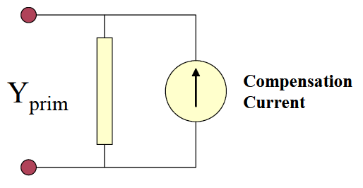
Figure 16. Compensation Current Model of PC Elements (one-line)
The Compensation current is the current that is added into the injection current vector in the main solver (see next section). This model accommodates a large variety of load models quite easily. The Load element models presently implemented are:
1.Constant P and constant Q load model: generically called constant power load model. It is the model most commonly used in power flow studies. It can suffer convergence problems when the voltage deviates too far from the normal range;
2. Constant Z (or constant impedance) load model: P and Q vary by the square of the voltage. This load model usually guarantees the convergence in any loading condition. The model is essentially linear;
3. Constant P and quadratic Q load model: the reactive power, Q, varies quadratically with the voltage (as a constant reactance) while the active power, P, is independent from the voltage, somewhat like a motor;
4. Exponential load model: the voltage dependency of P and Q is defined by exponential parameters (see CVRwatts and CVRvars). This model is typically used for Conservation Voltage Reduction (CVR) studies. It is also used for general distribution feeder load mix models when the exact behavior of loads is not known;
5. Constant I (or constant current magnitude) load model: P and Q vary linearly with the voltage magnitude while the load current magnitude remains constant. This is a common in distribution system analysis programs;
6. Constant P and fixed Q2 (Q is a fixed value independent of time and voltage);
7. Constant P and quadratic Q: Q varies with square of the voltage
8. ZIP load model: P and Q are described as a mixture of constant power, constant current and constant impedance load models whose contribution is defined by coefficients (see ZIPV).
Loads can be exempt from loadshape mulitipliers.All load models revert to constant impedance constant Z load model outside the normal voltage range (that can defined by the user, see Vminpu and Vmaxpu) in an attempt to guarantee convergence even when the voltage drops very low. This is important for performing annual simulations.
See PC Elements in the OpenDSS TechNotes and documentation section for further information and application examples