OpenDSS Documentation

Python to OpenDSS Interface for Modeling Control Systems

The detailed syntax for interfacing with the Open Distribution System Simulator (OpenDSS) is here presented in Python scripting language, emphasizing Distribution Management System (DMS) control applications. These tools are designed to form the building blocks of a sandbox module, to facilitate

simulating custom control methods. 

Set up the OpenDSS Interface for Simulation

The Python module win32com.client provides access to the OpenDSS COM module.

import win32com.client

dssObj = win32com.client.Dispatch(“OpenDSSEngine.DSS”)

The COM module has a variety of interfaces, and creating variables to access them directly is handy.

dssText = dssObj.Text

dssCircuit = dssObj.ActiveCircuit

dssSolution = dssCircuit.Solution

dssElem = dssCircuit.ActiveCktElement

dssBus = dssCircuit.ActiveBus

To load a circuit file into OpenDSS, use the text interface. This interface can also be used to execute any ordinary OpenDSS command via the COM interface.

dssText.Command = ”compile ‘testCircuit.dss’”

Get and Set the States of Controlled Elements

Capacitors

A capacitor’s full name will be “capacitor.capacitorname1”. To access a capacitor, send the second part of its name to the capacitor interface to make it the active capacitor. Then any action taken in the capacitor interface will refer to that capacitor. These commands access the current state of a capacitor:

dssCircuit.Capacitors.Name = “capacitorname1”

currentState = dssCircuit.Capacitors.States[0]

The zero index is here used because the states function returns an array of capacitor states, for each step. If steps are not used, the returned value will be a tuple, or array, of length 1. Note that this array is not always accurate for versions of OpenDSS before v7.6.4.53.

To set the state of another capacitor to 1, use the following lines of code:

dssCircuit.Capacitors.Name = “capacitorname2”

dssCircuit.Capacitors.States = (1,)

The states variable must take a tuple and not just an integer.

Regulators

Controlling a regulator really means controlling a transformer tap. The transformer will be named in the format “transformer.transformername1”. To access this transformer, use the transformer interface to make it active by passing the second part of the full name. Then any action taken to the transformer interface will affect that particular transformer, including changing the regulator tap.

Some arithmetic is required, to get and set the tap as an integer in the range [-16, 16]. The following code finds the current tap value and then sets the tap to 6, using the common 0.00625 tap width.

dssCircuit.Transformers.Name = “transformername1”

dssCircuit.Transformers.wdg = 2

currentTap = float(dssCircuit.Transformers.Tap - 1) / 0.00625

newTap = 6

dssCircuit.Transformers.Tap = 1 + newTap * 0.00625

A regulator can be controlled less directly by just controlling the forward vreg setting on an ordinary regulator controller and allowing the regcontrol element to do the control work itself. This can be done using the regcontrol interface, as shown by the following code. Normally the vreg setting is given on a 120 V base.

dssCircuit.RegControls.Name = “regcontrol3c”

dssCircuit.RegControls.ForwardVreg = 124

Switches

To use a line as an open switch, change “bus2” to some new bus name. To close it again, restore the old bus name.

switchName = “Line.L234”

dssCircuit.Lines.Name = switchName.split(".")[1]

# Open the switch

oldBusName = dssCircuit.Lines.Bus2

dssCircuit.Lines.Bus2 = "__opened__" + oldBusName

# Close the switch

oldBusName = dssCircuit.Lines.Bus2

dssCircuit.Lines.Bus2 = \

oldBusName[oldBusName.index("__opened__") + 10:]

In the previous example, __opened__ is prepended to the bus name and removed when the switch is reclosed.

Loads

The loads interface works identically to that of the capacitors, transformers, and switches. Set the active element with the Name field, and change kW, kVAr, and pf as required. The following section of code shows doubling the kVAr of a given load.

loadName = “Load.Load1”

dssCircuit.Loads.Name = loadName.split(“.”)[1]

oldkvar = dssCircuit.Loads.kvar

dssCircuit.Loads.kvar = 2 * oldkvar

Generators

Generators also have a COM interface. For variables for this and other elements that are not accessible via the COM interface, see “Elements without a COM interface” below. Again, set the active element with the Name field, and change kW, kVAr, and pf as required. The following code shows increasing the generation by 5 kW.

genName = “Generator.gen1”

dssCircuit.Generators.Name = genName.split(“.”)[1]

oldkw = dssCircuit.Generators.kw

dssCircuit.Generators.kw = oldkw + 5

Elements without a COM interface

Any property from any element can be accessed using the properties interface. For example, to change the model of a generator, execute the following code.

genName = “Generator.gen1”

dssCircuit.setActiveElement(genName)

dssElem.Properties(“model”).Val = 3

Note that PV systems and energy storage systems do not yet have a COM interface, but their properties can be changed in this way.

PV systems

Active and reactive power are the primary control variables for PV systems. Active power is set as the property pctPmpp, which caps the kW output as a percentage of rated. Reactive power can be changed by setting the kvar value, for constant var mode, or by setting the PF property, for constant power factor mode. Since this element does not have a COM interface, set these properties as described in “Elements without a COM interface” above.

pvName = “PVsystem.pv1”

dssCircuit.setActiveElement(pvName)

previousQ = dssElem.Properties(“kvar”).Val

dssElem.Properties(“kvar”).Val = 25

PV systems can be controlled by InvControl elements to perform some basic control functions. These must be disabled for manual control, as described below in “Existing control elements,” or they may have their properties adjusted similarly to PV systems for a higher-level control paradigm.

Energy storage systems

The state of the storage element, which may be charging, idling, or discharging, is the key controlled variable. Other important variables are charging and discharging rates and reactive power control. Another method is to specify the kW flow directly, which may be positive, negative, or zero, to indicate discharging, charging, or idling, respectively. To monitor in these low level ways, it is essential to disable any associated energy storage controllers, as described in “Existing control elements” below, and set the dispatch mode of the storage element to external. Following is example code which sets dispatch mode to external, specifies the state to discharge and discharge rate to 81%, and reads the percent of energy which is presently stored.

storageName = “storage.st1”

dssCircuit.setActiveElement(storageName)

dssElem.Properties(“DispMode”).Val = “EXTERNAL”

dssElem.Properties(“state”).Val = “DISCHARGING”

dssElem.Properties(“%Discharge”).Val = 0.81

energyStored = dssElem.Properties(“%stored”).Val

Other options for energy storage elements involve editing the parameters of built-in dispatch modes or those of an associated storage controller element. However, if these modes are active, they will override any changes to the low-level parameters such as kW and pf.

Even if an energy storage controller is disabled, it may have already changed some variables in the storage element. To avoid this, just remove the storage controller from the original OpenDSS file or manually reset the parameters that have been changed.

For reactive power control, as of OpenDSS 7.6.4.44, the kvar setting for storage elements does not work as consistently as the power factor setting.

Existing control elements

A variety of control elements exist built-in to OpenDSS. So long as they remain enabled, they will continue to execute their control functions, overriding any manual changes. Disable them by changing the “enabled” property just like any other. This example shows disabling a regulator controller element, so that the user can control the transformer tap without interference.

dssCircuit.setActiveElement(“regcontrol.regctr1”)

dssElem.Properties(“enabled”).Val = False

It is also possible to disable all control elements by turning control mode of the simulator off.

dssSolution.ControlMode = -1

Measure and Monitor the System State

Control decisions will often be based on measured voltage, current, and active and reactive power at various places in the system.

Monitor Elements

Creating a monitor element is an excellent way to keep a record of important values throughout a time-based simulation, and save these to a file. See the OpenDSS manual for more information about setting these up in the OpenDSS script.

The following Python code is used to save all monitors and export monitorname1 to a csv file:

mName = “monitorname1”

dssCircuit.Monitors.SaveAll()

dssText.Command = "export monitors " + mName

However, it is not possible to read the values of a monitor in the middle of a simulation; use another method below for control decisions.

Bus Voltages

To measure a bus voltage for control purposes, first make it the active bus using the circuit interface. Then use the ActiveBus interface to retrieve the phase or sequence voltage magnitudes and phases.

dssCircuit.SetActiveBus(“sub_lsb”)

puList = dssBus.puVmagAngle

Following is a table of bus voltage commands and what exactly is returned:

Element Currents, Powers, and Voltages

To measure currents and powers for control purposes, use the circuit interface to make a given power delivery or power conversion element the active circuit element. Then use one or more commands on the ActiveElement interface to measure the appropriate quantities.

dssCircuit.SetActiveElement(“Line.L3”)

cplxPowers = dssElem.Powers

seqCurrents = dssElem.SeqCurrents

The following table shows many available commands to measure different current and power values. Some of the above voltage commands also apply to the terminals of a circuit element.

Execute System Simulation

A time-based simulation must be set up with an OpenDSS command in the original script, or with a COM interface text command.

set mode=daily stepsize=15m number=96

Once the solution is set up, the time-based simulation can be executed in OpenDSS with a single call to the Solution interface:

dssSolution.Solve()

However, DMS control applications require custom actions to be performed at varying places within the OpenDSS solution process. To avoid confusion, a discussion of the OpenDSS solution process is next, followed by example interface scripts to insert custom controls in various points of the process.

Overview of OpenDSS simulation process

The OpenDSS simulation process is illustrated in the flow chart of Figure 1. Each time step consists of three main parts. First, a solution with controls is completed unto convergence, shown by the large yellow box. Next, clean-up operations are done such as sampling monitors and updating the charge percentage of a storage element. Finally, if there is another time step, time is incremented and the loop begins again. Within the solve-with-control block, the small blue blocks depict the controller operations in OpenDSS. For the necessary number of control iterations, each control element is allowed to measure the results of the power flow and push actions to the control queue for operation after a delay. When all actions on the control queue have been completed and no further ones are added, or if the number of control iterations has exceeded the maximum, the solution with controls is considered finished.

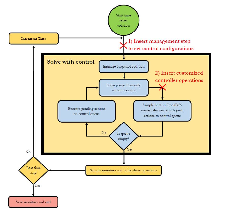
Figure 1: Flow chart of OpenDSS simulation process

Figure 1 also shows the two locations, marked by red X’s, where a user may want to insert control actions. Point (1) is the place for DMS-style control optimization settings, where the parameters for each control element can be set. Management tools can use the entire large solve-with-control block as a testing function to see what the results will be from any number of configurations.

To implement true customized control elements, which can push actions to the control queue, iterate over each control cycle, and interact with other controllers through timing setup, the user must insert functions at point (2) on the chart of Figure 1. This point is inside the control function and has the benefit of customized controller iterations, but decisions here cannot use the entire yellow box as a test unit without causing infinite recursion.

Management actions and control optimization

This example assumes that some sort of time-based simulation is already set up in the OpenDSS script file, such as a daily load shape with mode set to daily. The key is to find the original number of time steps and then run them one at a time, calling the custom control function once at each step.

originalSteps = dssSolution.Number

dssSolution.Number = 1

for ii in range(0, originalSteps):

controlFunction()

dssSolution.SolveSnap()

dssSolution.FinishTimeStep()

Setting the solution number to one causes the solve function to only run a single time step, and the new FinishTimeStep() function places the cleanup and increment actions at the end. Now the custom control function can make measurements and change control settings, even using SolveSnap() to

analyze possible configurations before setting the controls for the time step.

An important note about OpenDSS solutions

OpenDSS does not in any way reset to a previous configuration. The ending state of a circuit after a simulation, even if time does not advance, is retained every time. So if at 1 PM a capacitor controller operates to close a capacitor, running the simulation again, even at 1 PM, will not have the same effect unless the user manually opens the capacitor to restore it to its original state before running the simulation. This way of operation is critical to the performance of OpenDSS, but must be kept in mind when doing control optimizations. Care must be taken to reset the circuit to its original state after doing a test solution.

Emulate the control iteration loop

To implement a true custom control element, it is necessary to replace the SolveSnap() command above, which corresponds to the large yellow block in Figure 1, with an emulation to allow access at point (2). This is done with code similar to below.

dssSolution.InitSnap()

iteration = 0

while not dssSolution.ControlActionsDone:

dssSolution.SolveNoControl()

customControlLoop()

dssSolution.CheckControls()

iteration += 1

if iteration > dssSolution.MaxControlIterations:

break

Now at each control iteration, the custom control loop will be run before any OpenDSS controls. A discussion of adding control queue functionality follows.

Access the control queue

The control queue provides a higher-detailed level management of the control iterations. OpenDSS performs many control iterations, solving the power flow each time, until all pending actions have been completed and no control devices push new actions to the control queue. For more information about the control queue and how it interfaces with COM, see the document “OpenDSS CtrlQueue Interface.pdf” in the OpenDSS docs. Here is an example of pushing two control actions to the control queue. In Python, it may be helpful to map the device handle to a Python function using a dictionary. In this example, actionFunction1 and actionFunction2 are two functions that take actionCode as a single argument.

def actionFunction1(actionCode):

print “function 1: action code is “ + str(actionCode)

def actionFunction2(actionCode):

print “function 2: action code is “ + str(actionCode)

actionMap = {0: actionFunction1, 1: actionFunction2}

h = 1

s = 15

actionCode = deviceHandle = 0

dssCircuit.CtrlQueue.Push(h, s, actionCode, deviceHandle)

s = 30

actionCode = deviceHandle = 1

dssCircuit.CtrlQueue.Push(h, s, actionCode, deviceHandle)

However, OpenDSS will not handle these actions themselves. OpenDSS will simply push the device handle and action code to the action list when the time comes for them to be executed. To catch these actions, after CheckControls() has been run, use the dssCircuit.CtrlQueue class on the COM module, as demonstrated below. Assume that the previous block of code is inside customControlLoop() and that this code would be part of the block with the while loop on the previous page.

customControlLoop()

dssSolution.CheckControls()

while dssCircuit.CtrlQueue.PopAction != 0:

deviceHandle = dssCircuit.CtrlQueue.DeviceHandle

actionCode = self.dssCircuit.CtrlQueue.ActionCode

actionFunction = actionMap[deviceHandle]

actionFunction(actionCode)

By stepping through the control iterations, the user can call his custom function at each control iteration, push actions to the control queue, and handle them as they are pushed back by OpenDSS. In this framework, custom control actions happen alongside internal OpenDSS controls. The framework also allows for adding delays to control actions in the custom loop, which is typical behavior for conventional control schemes.

Full Simulation Example

This example shows the code to load a circuit file, set up a daily simulation, and perform custom control functions at both points in Figure 1.

# Simulation example using OpenDSS COM interface

import win32com.client

dssObj = win32com.client.Dispatch("OpenDSSEngine.DSS")

dssText = dssObj.Text

dssCircuit = dssObj.ActiveCircuit

dssSolution = dssCircuit.Solution

dssElem = dssCircuit.ActiveCktElement

# Load the circuit and set up the daily simulation

dssText.Command = r"compile 'master.dss'"

dssText.Command = r"compile 'setupDaily.dss'"

dssSolution.MaxControlIterations = 20

# Iterate through the time steps

originalSteps = dssSolution.Number

dssSolution.Number = 1

for stepNumber in range(originalSteps):

print "-- step " + str(stepNumber)

# as an example, measure the bus voltage and decide

# if cap control should be enabled or not.

# running a solve with control would also be possible here

# this is point (1) on Figure 1

dssCircuit.SetActiveBus("cap_bus")

capVolt = dssBus.puVmagAngle[0]

dssCircuit.setActiveElement("capcontrol.cc1")

if capVolt > 0.94:

dssElem.Properties("enabled").Val = True

else:

dssElem.Properties("enabled").Val = False

# Run the solve with control loop

dssSolution.InitSnap()

iteration = 0

while not dssSolution.ControlActionsDone:

dssSolution.SolveNoControl()

# This is point (2) on Figure 2

# as an example, push two action functions to the

# control queue. They will both update the kVAr of

# PV systems. The first will be delayed by 15 seconds,

# and the second by 30 seconds.

# These are only pushed on the first iteration,

# otherwise the solution will never converge!

def actionFunction1(actionCode):

dssCircuit.setActiveElement("pv1")

dssElem.Properties(“kVAr”).Val = 25 + 4 * actionCode

def actionFunction2(actionCode):

dssCircuit.setActiveElement("pv2")

dssElem.Properties(“kVAr”).Val = 15 + 4 * actionCode

actionMap = {0: actionFunction1, 1: actionFunction2}

h = 1

s = 15

actionCode = deviceHandle = 0

if iteration == 1:

dssCircuit.CtrlQueue.Push(h, s, actionCode,deviceHandle)

s = 30

actionCode = deviceHandle = 1

if iteration == 1:

dssCircuit.CtrlQueue.Push(h, s, actionCode,deviceHandle)

# with this command, OpenDSS pushes active to queue

dssSolution.CheckControls()

# if there are any actions which OpenDSS is calling to

# be handled now, this loop will do so.

while dssCircuit.CtrlQueue.PopAction != 0:

deviceHandle = dssCircuit.CtrlQueue.DeviceHandle

actionCode = self.dssCircuit.CtrlQueue.ActionCode

actionFunction = actionMap[deviceHandle]

actionFunction(actionCode)

iteration += 1

if iteration >= dssSolution.MaxControlIterations:

print "exceeded max iterations!"

break

dssSolution.FinishTimeStep() # cleanup and increment time

Early Binding on COM Interface

Python by default uses late binding for COM interfaces, which means that each property and method will be found via a time-consuming lookup process. In contrast, early binding greatly improves time performance of the COM interface and may be helpful for complex simulations. Note that all object properties become casesensitive when early binding is used.

To use early binding in the following two first lines of code:

import win32com.client

dssObj = win32com.client.Dispatch("OpenDSSEngine.DSS")

Instead use the following code, which takes advantage of the makepy package to do the early binding on the OpenDSSEngine interface.

import win32com.client

from win32com.client import makepy

import sys

sys.argv = ["makepy", "OpenDSSEngine.DSS"]

makepy.main()

dssObj = win32com.client.Dispatch("OpenDSSEngine.DSS")

Explore Other Resources

Information about the capabilities of OpenDSS can be found in the OpenDSS help, as well as the manual and other documentation and examples available at https://www.epri.com/pages/sa/opendss?lang=en

Once the OpenDSS COM server is registered on a computer, Microsoft Excel’s VBA object browser is an excellent way to explore the possibilities in the OpenDSS COM server. From Excel, press Alt+F11, then choose Tools > References, and select the OpenDSSEngine. Press F2 to open the object browser, and select the OpenDSSEngine from the project library drop-down combo box. The available classes will be on the left, and the members will be listed to the right.

For more information about Python, see https://docs.python.org/2/