OpenDSS Documentation

Time measurement in OpenDSS

Introduction

To improve the performance of OpenDSS for Quasi‐Static Time Series (QSTS) simulations project, it has become necessary to add a timer functionality to OpenDSS in order to record the time required for the different segments of the power flow solution. The power flow solution involves three main stages as follows:

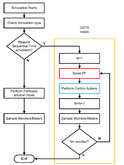
Figure 1. General diagram describing the Power Flow solution in sequential‐time simulations (OpenDSS)

• The Solution stage: In this stage the program will solve the circuit power flow for one time step. This stage is an iterative stage that will update the injected currents from loads and generators until the circuit solution converges. This stage also includes the control actions performed by the controls such as Inverter controls, capacitor controls, regulators, among others.

• The Sampling stage: the Solution stage is followed by a routine for sampling the meters and monitors distributed by the user on the circuit. This action involves dynamic memory allocations and disk file I/O. If there are no monitors/meters defined on the circuit this stage should not add much time to the Solution stage.

• The Simulation stage: This stage contains the both stages described above and includes an iteration counter defined by the parameter number in OpenDSS, which causes OpenDSS to perform the power flow solution and sampling number times as specified by the user. This is how sequential‐time simulations and dynamic simulations are executed.

These 3 stages report different times since each one incorporates part of the process of the simulation routine. This suggests that it is necessary to have a different timer for each part as shown in Figure 1.

As can be seen in Figure 1, the sequential‐time solution process has the 3 stages clearly identified. However, the way these are integrated in the algorithm is not the same since stage 3 contains stages 1 and 2. This feature makes it necessary to create 3 different timers for measuring the entire solution process in its different stages.

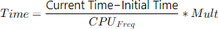
The 3 timers created for measuring the time of each stage rely on the windows API to measure the elapsed time based on processor ticks. The tick count is later processed using the processor’s frequency to translate ticks into time units (nanoseconds, microseconds, milliseconds) as needed. The expression used for this translation is as follows:

                  (1)

In expression (1) the Initial Time is taken when the process starts and the current time is the time at the moment the calculation is completed. Since the time is in terms of processor ticks these values are absolute and the current time will be always greater that the initial time. After dividing this value by the processors frequency (CPU Freq) the time obtained will be in the lowest time units possible with the processor. Considering that nowadays processor CPU frequencies are expressed in GHz, this unit will be in tenths of a nanosecond.

To convert this to a more practical time, the results are multiplied by a compensation factor, Mult. The value of this factor can be changed depending on the time units required for this project. For timing QSTS simulations, the most accurate unit for expressing the time required for each stage will be in

microseconds, a time unit that requires mult=1e6.

The features of each of the 3 timers are described in TABLE I.

These timers are available through the multiple interfaces available in OpenDSS (Executable, COM and Direct DLL). Additionally, two of these timers can be captured at each time step using monitors in mode 5. The values of the timers Process Time and Step Time are saved in Monitor channels 12 and 13

(SolveSnap_uSecs and TimeStep_uSecs respectively). It is not important where the mode‐5 monitor is placed in the circuit; it is common to put in on the main Vsource. It simply needs to exist when the monitors are sampled. An explanation of how to access the timers in the various forms of OpenDSS

follows:

Accessing the timers using the standalone (Executable) interface

In the Executable version the user will have access to the timers by using the options ProcessTime, TotalTime and StepTime as follows:

The return values are display in the Result window, as with all Get commands.

The following example shows how to query the timers using an OpenDSS script (the file master.dss is the master script of the IEEE 8500 node feeder [1]).

Example 1

Compile (master.dss)

New Energymeter.m1 Line.ln5815900-1 1

New monitor.SysVars element=Line.ln5815900-1 terminal=1 mode=5 ! This monitor records the timers using a CSV file

Set Maxiterations=20 ! Sometimes the solution takes more than the default 15 iterations

Set TotalTime=0 ! The total timer is set to 0

Solve mode=time !--- this mode automatically samples Monitors and Meters after the 1 snapshot solution

get ProcessTime ! Request the time required to perform the latest solution without sampling meters

get StepTime ! Request the time required to perform the latest solution including sampling meters

solve !--- do another time step

Export Monitor SysVars

get TotalTime ! At this point The TotalTime timer will report the time required to perform 2 time steps

After running this script the user will find a file in the projects folder called IEEE8500_Mon_sysvars.csv,bthis file will report the values presented in TABLE II (Columns 7 to 13).

As can be seen in TABLE II the last two columns of the report show the time required for solving the circuit power flow for the time step in column 12, and then the total time for the time step including the time required for sampling meters in column 13. Using the information provided by these registers it can be inferred that the time required for sampling the existing meters is 2 microseconds, or to be more exact, 1.86 microseconds.

Additionally, in the results window of OpenDSS will appear the value 385592.9139, which is the value stored in the TotalTime timer and can be calculated by adding the time registered for the TimeStep timer at each simulation step. These values depend on the CPU frequency and can change from one PC

to another according to their characteristics. In this particular case, the computer used was an Intel(R) Core(TM) i5‐5200U CPU @ 2.20GHz.

Accessing the update from the COM interface

In the COM interface 3 new properties have been included in the Solution Interface: Process_Time, Time_of_Step and Total_Time. To illustrate the use of these properties using the COM interface the following example is proposed (MATLAB):

Example 2

clc;

clear;

[DSSStartOK, DSSObj, DSSText] = DSSStartup;

myDir = cd;

if DSSStartOK

DSSText.command = ['Compile (',myDir,'\master.dss)'];

DSSText.Command = 'New monitor.SysVars element=Line.ln5815900-1

terminal=1 mode=5';

% Set up the interface variables

DSSCircuit = DSSObj.ActiveCircuit;

DSSSolution = DSSCircuit.Solution;

% Starts simulation

DSSSolution.Total_Time= 0;

DSSText.Command = 'Set Maxiterations=20';

DSSText.Command = 'Set mode=time';

DSSSolution.Solve;

Time0 = DSSSolution.Process_Time

Time1 = DSSSolution.Time_of_Step

DSSSolution.Solve;

DSSText.command = 'Export Monitors SysVars';

Total_Time = DSSSolution.Total_Time

else

a='DSS Did Not Start'

disp(a)

end

After running the latest script, the results should be very nearly the same as the ones described in section (a). In this case, the time required to solve the first iteration of the simulation are stored at variables Time0 and Time1 for the Process Time and Time Step timers respectively, and the total time for the simulation (Total Time timer) is stored at Total_Time.

Accessing the update from the DIRECT DLL interface

In the Direct DLL interface, 4 new parameters have been included in the SolutionF Interface: 24 (Process_Time), 25 (Total_Time read), 26 (Total_Time Write) and 27 (Time_Step). As in the cases above, the use of these parameters will be illustrated using an example (MATLAB).

Example 3

Process_Time = 24;

Total_Time_Read = 25;

Total_Time_Write = 26;

Time_of_Step = 27;

Start = 3;

Solve = 0;

% Connect to the DLL

%addpath(fullfile(pwd))

myDir = cd;

loadlibrary('OpenDSSDirect.dll',@DEngineProto);

calllib('OpenDSSDirect','DSSI',Start,0);

calllib('OpenDSSDirect','DSSPut_Command',['compile (',myDir,'\master.dss)']);

calllib('OpenDSSDirect','DSSPut_Command','New monitor.SysVars

element=Line.ln5815900-1 terminal=1 mode=5');

calllib('OpenDSSDirect','DSSPut_Command','set mode=time maxiterations=20');

calllib('OpenDSSDirect','SolutionF',Total_Time_Write,0);

calllib('OpenDSSDirect','SolutionI',Solve,0);

Time0 = calllib('OpenDSSDirect','SolutionF',Process_Time,0)

Time1 = calllib('OpenDSSDirect','SolutionF',Time_of_Step,0)

calllib('OpenDSSDirect','SolutionI',Solve,0);

calllib('OpenDSSDirect','DSSPut_Command','Export monitor SysVars');

Total_Time = calllib('OpenDSSDirect','SolutionF',Total_Time_Read,0)

% Disconenct the DLL

unloadlibrary 'OpenDSSDirect'

The file DEngineProto.m is a prototype file created manually to identify the interfaces of the DLL in MATLAB, this file is provided with the MATLAB example at the OpenDSS website and can be updated manually by the user. The components and interfaces of this DLL are described at the DLL’s user manual.

References

[1] R. F. Arritt and R. C. Dugan, "The IEEE 8500‐node test feeder," in 2010 IEEE PES Transmission and Distribution Conference and Exposition, 2010, pp. 1‐6. 

Acknowledgement

This feature in OpenDSS was requested and funded by the US DOE SuNLaMP project through Sandia National Laboratory and the National Renewable Energy Laboratory to allow comparisons of various techniques to speed up Quasi‐static Time Series (QSTS) simulations in OpenDSS.