OpenDSS Documentation

Diakoptics based on Actors (A-Diakoptics) combines two computing techniques from different engineering fields: Diakoptics and the actor model. Diakoptics is a mathematical method for tearing networks. The actor model is used to coordinate the interaction between sub-circuits.

A-Diakoptics is a technique that seeks to simplify the power flow problem to achieve a faster solution at each simulation step. Consequently, the total time reduction when performing QSTS will be evident at each simulation step with A-Diakoptics.

This technique has been implemented in OpenDSS in version 9.4 using a simplification that will be explained later in this document. The suite integrated in version 9.4 includes automated and manual circuit tearing among other tools to execute and debug the method step by step. Since the simplification implemented in OpenDSS is relatively new, we will continue to improve the suite in time.

The simplified A-Diakoptics solution method

Initially proposed by Gabriel Kron and later used and modified by other authors [1, 2]. Diakoptics is a technique for tearing large physical circuits into several sub-circuits to reduce the modeling complexity and accelerate the solution of the power flow problem using a computer network. Each computer will handle a separate piece of the circuit to find a total solution. Using modern multi-core computers this technique can be used for accelerating QSTS simulations, in OpenDSS, by using the actor model as a framework for coordinating the interactions between the distributed pieces proposed in Diakoptics [3, 4].

A-Diakoptics uses the parallel processing suite inside OpenDSS to allocate and solve the separate pieces of the interconnected circuit. A-Diakoptics was proposed initially in 2015 [5, 6] and utilizes the power flow solution method proposed in OpenDSS for the analysis.

The power flow problem in OpenDSS

While the power flow problem is probably the most common problem solved with the program, the OpenDSS is not best characterized as a power flow program. Its heritage is from general-purpose power system harmonics analysis tools. Thus, it works differently than most existing power flow tools. This heritage also gives it some unique and powerful capabilities for modeling complex electrical circuits. The program was originally designed to perform nearly all aspects of distribution planning for distributed generation (DG), which includes harmonics analysis. It is relatively easy to make a harmonics analysis program solve a power flow, while it can be quite difficult to make a power flow program perform harmonics analysis. To learn more about how the algorithm works for the power flow problem, see “Putting It All Together” below. [Where is this?]

The OpenDSS program is designed to perform a basic distribution-style power flow in which the bulk power system is the dominant source of energy. However, it differs from the traditional radial circuit solvers in that it solves networked (meshed) distribution systems as easily as radial systems. It is intended to be used for distribution companies that may also have transmission or sub transmission systems. Therefore, it can also be used to solve small- to medium-sized networks with a transmission-style power flow.

Nearly all variables in the formulation result in a matrix or an array (vector) to represent a multiphase system. Many of the variables are complex numbers representing the common phasor notation used in frequency-domain ac power system analysis.

OpenDSS uses a standard Nodal Admittance formulation that can be found documented in many basic power system analysis texts. The Arrillaga and Watson textbook is useful for understanding this because it also develops the admittance models for harmonics analysis similarly to how OpenDSS is formulated.

A primitive admittance matrix, Yprim, is computed for each circuit element in the model. These small matrices are used to construct the main system admittance matrix, Ysystem, that knits the circuit model together. The solution is mainly focused on solving the nonlinear system admittance equation of the form:

IPC(E) = Compensation currents from Power Conversion (PC) elements in the circuit 

The currents injected into the circuit from the PC elements, IPC(E), are a function of voltage as indicated and represent the nonlinear portion of the currents from elements such as Load, Generator, PVsystem, and Storage.

There are several ways this set of nonlinear equations could be solved. The most popular way in OpenDSS is a simple fixed point method that can be written concisely [7]:

 n=0,1,2 ... until converged

From here it can be inferred that every time an expression like the following is found:

there is an OpenDSS solver, called an actor in OpenDSS’ parallel processing suite, and this is the basis for the A-Diakoptics analysis.

Simplified A-Diakoptics

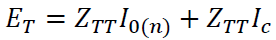
An initial form of A-Diakoptics was developed in [5, 6]. From there, the general expression for describing the interactions between the actors (sub-circuits) and the coordinator is as follows:

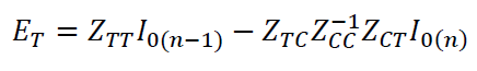
ET is the total solution of the system (the voltages in all the nodes of the system). I0 is the vector containing the currents injected by the PC elements, and the time instants n and n +1 are discrete time instants to describe the different times in which the vector of currents is calculated [6]. ZTT is the trees matrix and contains the admittance matrixes for all the sub-circuits that contained in the interconnected system after the partitioning. The form of ZTT is as follows:

The sub-circuits contained in ZTT are not interconnected in any way. The connections are through external interfaces that define the relationship between them. ZTC, ZCT and ZCC are interfacing matrixes for interfacing the separate subsystems using a graph defined by the contours matrix (C) as described in [6, 8]. ZTTI0(n-1) corresponds to the solutions delivered when solving the sub-systems and ZTCZCC-1ZCTI0(n) is the interconnection matrix to find the total solution to the power flow problem.

As can be seen at this point, the form of ZTT proposes that multiple OpenDSS solvers can find independent partial solutions that when complemented with another set of matrixes, can calculate the voltages across the interconnected power system. However, in this approach the interconnection matrix is a dense matrix that operates on the injection currents vector provided by the latest solution of the sub-systems.

Nowadays, sparse matrix solvers are very efficient and to operate with a dense matrix is not desirable. The aim in this part of the project is to simplify the expression that defines the interconnection matrix to find a sparse equivalent that can be solved using the KLUSolve module already employed in OpenDSS.

Assuming that the times in which the sub-systems are solved, and the interconnection matrix is operated are the same and fit into the same time window (ideally), A-Diakoptics can be reformulated as:

Additionally, in OpenDSS the interconnected feeder is solved using:

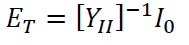
Where YII is the YBus matrix that describes the interconnected feeder. Equating the two previous equations the expression results in:

This new expression can be taken to the admittance domain since ZTT is built using the YBus matrixes that describe each one of the sub-systems created after tearing the interconnected feeder [5, 6]. The new equation is reformulated as:

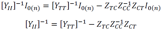
Then the interconnection matrix can be reformulated as:

This new formulation proposes that the interconnection matrix is equal to an augmented representation of the link branches between the sub-systems. To support this conclusion take the simplification proposed by Happ in [8] where:

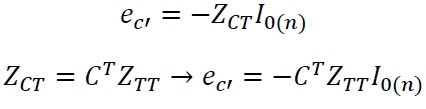
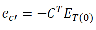
This expression is similar to the partial solution formulation of the Diakoptics equation but including the contours matrix, then if the partial solution is called ET(0) it is possible to say:

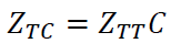
On the other hand, ZTC, which is the non-conjugate transposed of ZCT, is calculated as follows:

Replacing the new equivalences for ZCT and ZTC the equation proposed in (*) is reformulated as follows:

Or in terms of sparse matrices:

Where:

The new equation described in (2) establishes that the same actor can calculate its partial and complementary solutions using information calculated using the interconnection matrix ZCC. ZCC is a small matrix that contains the information about the link branches and the calculation of Ic does not represent a significant computational burden in medium and large-scale circuits. With this approach, all the matrix calculations are made using sparse matrix solvers, reducing the computational burden.

Using the A-Diakoptics suite in OpenDSS

The A-Diakoptics suite is an instruction set for driving simulations using A-Diakoptics in OpenDSS. This instruction set is available from version 8.5 and later. The instructions are as follows:

Circuit partitioning

After activating A-Diakoptics OpenDSS will deliver an output describing the result of the initialization. Consider the following lines of code for enabling A-Diakoptics using 4 sub-circuits (the circuit has been compiled and solved in snapshot mode previously):

set Num_Subcircuits=4

set ADiakoptics=True

If the partitioning and initialization of the circuit was correct, the output from OpenDSS will be as shown in Figure 1.

Figure 1. Circuit partitioning successful

As can be seen in Figure 1, the summary window will display all the steps carried out to initialize A-Diakoptics including the partitioning statistics (see partitioning statistics). At this point the system is ready to solve in A-Diakoptics mode. The following considerations need to be taken:

1. All monitors or energy meters can be created in actor 1. Actor 1 is the simulation coordinator, and it hosts Y4 and the vectors for calculating Ic. Actor 1 also hosts the admittance matrix of the interconnected circuit.

2. Actor 1 is the simulation coordinator; the others are slaves of the coordinator.

3. The number of actors depends on the number of sub circuits configured by the user. If the number of sub-circuits set by the user overpasses the number of CPUs – 2 in the local PC, the Initialization algorithm will force the number of sub-circuits to the number of CPUs – 2.

4. The CPUs are assigned automatically. If the user wants a better performance (e.g., 1 thread per Core) it is necessary to do the redistribution manually.

5. The algorithm is available for all the OpenDSS compilations: EXE, COM, and DLL. It is fully operational for all QSTS and direct solution modes.

Error messages

The A-Diakoptics initialization is a complex process and has multiple moving pieces that may cause an error in the initialization, making the initialization unsuccessful and aborting A-Diakoptics. Sometimes when creating the sub-circuits, one or more circuits cannot be solved, either because the circuit is invalid, or something is missing. In this case the message at the summary window in OpenDSS is as follows:

A-Diakoptics initialization summary:

- Creating Sub-Circuits...

6 Sub-Circuits Created

- Indexing link branches...Done

- Setting up the Actors...Error

One or more sub-systems cannot be compiled

One or more errors found

In this case the A-Diakoptics initialization failed and as a result, A-Diakoptics was not enabled.

OpenDSS uses MeTIS for the circuit partitioning. Sometimes MeTIS suggests a PD element different from a Line as a link branch, which is an error. In that case the output at the summary window will be:

A-Diakoptics initialization summary:

- Creating Sub-Circuits...

6 Sub-Circuits Created

- Indexing link branches...Done

- Setting up the Actors...Done

- Building Contours...Error

One or more link branches are not lines

One or more errors found

Again, the A-Diakoptics initialization failed and A-Diakoptics was not enabled. In this case the best solution is to propose a different number of sub-circuits until a valid partitioning is achieved. The partitioning can be validated using the partitioning statistics information.

Partitioning statistics

After a successful circuit partitioning OpenDSS will calculate some statistics to help the user to understand and estimate what to expect from the circuit tearing. There are 3 indicators delivered by OpenDSS called the circuit reduction, the maximum imbalance, and the average imbalance.

The circuit reduction is the relationship between the number of nodes in the interconnected circuit and the largest sub-circuit created after partitioning the circuit. The circuit reduction is calculated as follows:

It is the largest sub-circuit that will take longer to solve (normally), determining the total time required for solving a simulation step. 

The maximum imbalance and the average imbalance are 2 metrics oriented to illustrate the level of balance between sub-circuits. The maximum imbalance is calculated considering the relationship between the sizes of all the sub-circuits and the largest sub-circuit after the partitioning. 

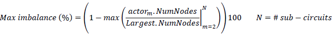
The average imbalance is the average of the all the imbalances considering the largest sub-circuit as reference.

The aim with these metrics is to keep them as low as possible after partitioning the circuit. Ideally, the average and maximum imbalances should be 0. However, that may happen only in very special situations. If the maximum imbalance is lower than 50 % it means that the tearing is acceptable. For example, consider the following statistics after tearing the circuit using 4 sub-circuits:

Circuit reduction (%): 68.52

Max imbalance (%): 42.33

Average imbalance (%): 20.52

These statistics reflect that the circuit had a reduction greater than the 50% and the maximum imbalance is not perfect but is below 50%. In another scenario using only 2 sub-circuits, the output is as follows:

Circuit reduction (%): 46.34

Max imbalance (%): 13.64

Average imbalance (%): 6.818

The imbalance ratio is much better than when using 4 sub-circuits, however, the reduction ratio is lower. Finally, consider a partitioning using 5 sub-circuits in the same system, the output is as follows:

Circuit reduction (%): 60.95

Max imbalance (%): 94.04

Average imbalance (%): 48.67

In this case, the circuit reduction is not higher than using 4 sub-circuits and the maximum and average imbalances growth significantly, indicating that the circuit partitioning is not better using more partitions.

Actors’ distribution in memory

The new implementation of A-Diakoptics considers several implementations, these can be reviewed in Table 1.

The transport of data between memory is simplified by pointing the distributed solvers to actor’s 1 memory. While the injected current vectors for each solver is kept locally, the output of the solution algorithm (voltage) is read/write in the part of the solution of actor 1 matching the nodes of each subnetwork.

For example, consider a circuit model with 14 nodes that is torn into 2 sub-circuits. Actor 1 will contain the model representing the 14-node system, which has a vector for representing the injected currents and another one for the voltages at each node, which also represents the solution. Both vectors have 14 elements.

Assume that the sub-circuits have 7 nodes each, in that case, actor 2 containing the first subnetwork will read/write the solution for its zone from the voltage vector in actor 1 starting at position 1 to 7. Actor 3 containing the second subnetwork will then read/write the solution for its zone from the voltage vector in actor 1 starting at position 8 to 14. This concept is illustrated in Figure 2.

Avoiding complicated math when possible is crucial for reducing computational overhead in simulation time. Even when the math suggests steps including linear algebra, these can be simplified by giving them the correct physical interpretation within the computer algorithm. For example, the expression:

Suggests that the partial voltages found in a previous step (ET(0)) need to be multiplied by the vector C before operating with the inverse of ZCC, which has been calculated at the initialization. ZCC-1 is expected to be a small matrix, then, CTET(0) is a linear algebra operation intended to reduce the partial voltage vector into the number of ZCC. However, the physical meaning of this reduction is the voltage difference at the terminal of the link branches, used to calculate the current injections representing the interactions between sub-circuits in the context of the interconnected system as depicted in Figure 2.

In this case, it is faster to extract the voltages at the nodes of interest and perform a simple subtraction for building the result CTET(0) than operating 2 vectors. Similar implementations are made when coding the new algorithm in OpenDSS to reduce the implicit overhead when working in parallel.

The read/write operations from the distributed solvers (actors 2 and 3) into the solution space of actor 1 are done using pointers, removing the need for transporting data from actors > 2 into actor 1 through iterative routines.

The present state for controller implementation in OpenDSS needs to be considered in future projects when using A-Diakoptics. Controllers that produce changes in the local Y Bus matrix of the distributed solvers introduce an error that can be significant. One option is to rethink those controllers using current injection equivalents, or, to optimize the calculation of the interconnection matrix ZCC to recalculate it every time a control action requires it.

Monitors and meters also need extra work when monitoring DER such as ES and PV, since their control actions and state variable change in the context of the distributed solvers, but it is actor 1 (coordinator) the one that sample meters. This can be easily solved by adding an index to the actor containing the element of interest to the meters in actor 1, a change that can be implemented in future releases.

Figure 2. Distributed solvers pointing to actor 1 solution space

Test circuits for A-Diakoptics

In version 9.4, OpenDSS includes 6 test cases publicly available on the internet for illustrating the features of the A-Diakoptics implemented in this project. The test cases proposed are:

IEEE 13 bus test case, used for learning more about A-Diakoptics and for debugging, available at:

https://sourceforge.net/p/electricdss/code/HEAD/tree/trunk/Version8/Distrib/Examples/ADiakoptics/IEEE_13_Bus/.

IEEE 123 bus test case, used for learning more about A-Diakoptics and for understanding its behavior when using Y Bus modifying and current based controllers, available at: 

https://sourceforge.net/p/electricdss/code/HEAD/tree/trunk/Version8/Distrib/Examples/ADiakoptics/IEEE_123_Bus-G/

EPRI Circuit 5, for testing simulation performance, available at:

https://sourceforge.net/p/electricdss/code/HEAD/tree/trunk/Version8/Distrib/Examples/ADiakoptics/EPRI_Ckt5-G/.

EPRI Circuit 7, for testing simulation performance, available at:

https://sourceforge.net/p/electricdss/code/HEAD/tree/trunk/Version8/Distrib/Examples/ADiakoptics/EPRI_Ckt7-G/

EPRI Circuit 24, for testing simulation performance, available at:

https://sourceforge.net/p/electricdss/code/HEAD/tree/trunk/Version8/Distrib/Examples/ADiakoptics/ckt24/

Transmission and distribution case (combining IEEE 30 bus and EPRI circuit 5), for testing simulation performance based on simulation complexity simplification, available at: https://sourceforge.net/p/electricdss/code/HEAD/tree/trunk/Version8/Distrib/Examples/ADiakoptics/TnDSystem/.

These test systems include the commands and instructions to evaluate the performance of A-Diakoptics. The user can modify the cases at will to fulfill his simulation needs. Also, result tables and statistics are provided within the test cases. The details on the findings and experiments conducted with these test systems are presented in [11].

References

[1] G. Kron, "Detailed Example of Interconnecting Piece-Wise Solutions," Journal of the Franklin Institute, vol. 1, p. 26, 1955.

[2] G. Kron, Diakoptics: the piecewise solution of large-scale systems: Macdonald, 1963.

[3] C. Hewitt, "Actor Model of Computation: Scalable Robust Information Systems," in Inconsistency Robustness 2011, Stanford University, 2012, p. 32.

[4] C. Hewitt, E. Meijer, and C. Szyperski. (2012, 05-15). The Actor Model (everything you wanted to know, but were afraid to ask). Available: http://channel9.msdn.com/Shows/Going+Deep/Hewitt-Meijer-and-Szyperski-The-Actor-Model-everything-you-wanted-to-know-but-were-afraid-to-ask

[5] D. Montenegro, G. A. Ramos, and S. Bacha, "Multilevel A-Diakoptics for the Dynamic Power-Flow Simulation of Hybrid Power Distribution Systems," IEEE Transactions on Industrial Informatics, vol. 12, pp. 267-276, 2016.

[6] D. Montenegro, G. A. Ramos, and S. Bacha, "A-Diakoptics for the Multicore Sequential-Time Simulation of Microgrids Within Large Distribution Systems," IEEE Transactions on Smart Grid, vol. 8, pp. 1211-1219, 2017.

[7] R. Dugan. (2016, OpenDSS Circuit Solution Technique. 1. Available: https://sourceforge.net/p/electricdss/code/HEAD/tree/trunk/Version7/Doc/OpenDSS%20Solution%20Technique.docx

[8] H. H. Happ, Piecewise Methods and Applications to Power Systems: Wiley, 1980.

[9] H. Meyerhenke, P. Sanders, and C. Schulz, "Parallel Graph Partitioning for Complex Networks," in 2015 IEEE International Parallel and Distributed Processing Symposium, 2015, pp. 1055-1064.

[10] H. H. Happ, "Z Diakoptics - Torn Subdivisions Radially Attached," IEEE Transactions on Power Apparatus and Systems, vol. PAS-86, pp. 751-769, 1967.

[11] Advancing spatial parallel processing for QSTS: Improving the A-Diakoptics suite in OpenDSS. EPRI, Palo Alto, CA: 2021. 3002021419.