OpenDSS Documentation

To model a generic n-conductor line in OpenDSS, as well as any other software, requires the corresponding impedance matrix Z1 (or the sequence impedances Zl and ZO) as shown in Eq. 1. This is the classic approach adopted to model a line. In this case OpenDSS uses the Linecode class.

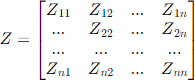eq. 1 

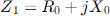
 Sequence Impedance :

However, in case the impedance data are not directly available, OpenDSS is able to produce the impedance matrix from the physical features of cables and line if provided. For this purpose, two following data are needed:

1)        The physical characteristics of the conductors (or cables) that constitute the line. Three classes can be adopted to input these data in OpenDSS: CNData – TSData (for cables) and WireData (for bare conductors)

2)        Cable-conductors disposition. For this purpose, the LineGeometry class is used in OpenDSS.

This technote will focus on the 2 classes adopted to describe concentric-neutral and tape shielded cables (i.e., CNData and TSData ). WireData and LineGeometry have already been described in this Help document).

CNDATA

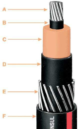
This class is adopted to describe concentric neutral cables. This cable owns his name by the neutral conductors that encircle the phase conductors as shown in Figure 1.

To describe a concentric neutral cable the CNData class in OpenDSS adopts the following properties:

                   
                         (a)                                                       (b)
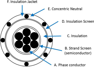
Figure 1 Structure of a Concentric Neutral Cable: a) From [1] b) simplified cross section (not in proportion)

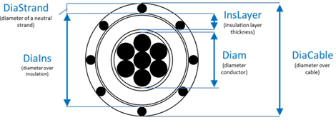
Figure 2 Main geometric properties in CNData class for a concentric neutral cable

Some of the previous geometric properties are also shown in Figure 2 in a cross section of a cable.

TSDATA

This class is adopted to describe the physical features of tape shielded cable as the one shown in Figure 3. The following properties can be defined in the TSData class:

(a)                                            (b)

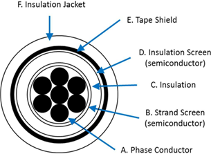
Figure 3 Structure of a Tape Shielded cable: a) From [2] b) simplified cross section (not in proportion)


Figure 4 Main geometric properties in TSData class for a tape shielded cable

PRACTICAL EXAMPLE: CONCENTRIC NEUTRAL CABLE

This section shows how to retrieve the data to model a concentric neutral cable . The same process can be repeated almost unchanged for tape shielded ones.

Let’s assume that the following cable needs to be modeled into OpenDSS.

Concentric neutral – Size=250 - Material=Aluminum – Neutral Size= 1/3

The geometric and electric properties required by the CNData class can be found in any manufacturer datasheet as shown in Figure 5 and summarized as follows:

DiaIns=1.16 in - DiaCable=1.29 in - k=13 - Insulation layer material: EPR (epsR=2.3) -                InsLayer=0.22 in

For the missing other resources such as [4] can be adopted. More precisely, for the phase conductors (250 AA with 19 strands) the following data were found (Appendix A in [4]):

insulation 220 mil (0.22 inch) – Insulation material= EPR

Figure 5 Features of a Concentric neutral cable (without jacket) – 250 Aluminum – 1/3 neutral, [3]

Phase Conductors: Diam=0.567 in – GMRac=0.0171 ft (or 0.205 in) – Rac=0.41 Ω/mi (or 0.0776 Ω/kft)

Regarding the stranded neutral (Size=14, No=13), always in Appendix A in [4], it was found:

Neutral: DiaStrand=0.064 in – Rstrand=14.87 Ω/mi (or 2.55 Ω/kft) GmrStrand=0.00208 ft (or 0.02496 in)

Consequently as all physical features are now defined the cable can be modeled into OpenDSS adopting the code shown in Figure 6.

Figure 6 OpenDSS code to model the concentric neutral – 250 Aluminum - 1/3 Neutral

Line Modeling: Primitive Impedance Matrix, Reduced Matrix, and Sequence Impedances

This section describes, adopting examples in OpenDSS, the differences between primitive, (Kron) reduced and sequence impedance. These are the three different “forms” of the line impedance matrix that can be adapted to model. This tech note does not have the ambition to provide a lecturer on the subject (as plenty of excellent books for the purpose) but simply to highlight some basic concepts leveraging the capability of OpenDSS in producing these models.

Let’s assume to model a three phase + neutral overhead line given by 4 AAC (i.e., All Aluminum Conductor) of American size 477. This line is one of the several modeled in the EPRI test case ckt242. The conductors features are describes below, their disposition is shown in Figure 7 and the corresponding code in OpenDSS is shown in Figure 8.

1.        Overall outside diameter=0.793 in

2.        GMR=0.3 in

3.        Rac=0.1968 Ohm/mile

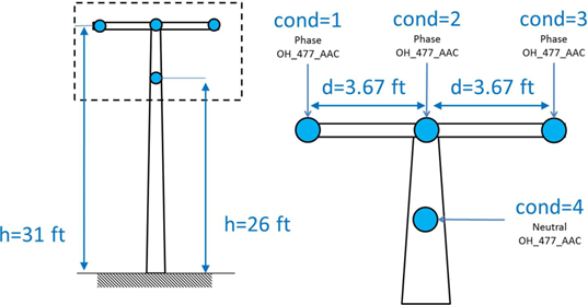
Figure 7 Modeled 3ph + neutral overhead line

Figure 8 OpenDSS code to model the line depicted in Figure 7

The main commands adopted in Figure 8 are explained as follows:

•earthmodel=Carson: OpenDSS produces the line load model based on the simplified Carson approach that typically is adopted for steady state study at nominal frequency (50- 60 Hz). The earth resistivity, “rho,” is generally specified with each Line definition and defaults to the commonly-assumed value of 100 m − Ω. More details on the impact of such model (over the others) are discussed in [5].

•WireData and LineGeometry: The WireData class is adopted (see User manual and OpendSS Help for more details) to describe the features of conductors while their placement on a pole or tower is detailed by the LineGeometry class. It is worth noticing that the WireData declaration should always be defined first. Otherwise OpenDSS cannot retrieve the conductor information referenced by the LineGeometry class.

•nconds=4 nphases=3: The line is defined by 4 physical conductors but only 3 phases. It means that the extra conductor (the cond=4 in the LineGeometry declaration in Figure 8) is considered as the neutral by OpenDSS . There can be multiple neutral wires.

•reduce=no: This means that the line model developed by OpenDSS is NOT Kron reduced.

•solve: This command solves the circuit. As no loads, sourcebus or lines are present it will simply calculates the line impedances. The line impedances can also be computed without executing a Solve command by using the Show command described next.

•show lineconstant freq=60 units=mi: This command will produce a CSV files reporting the line model developed by OpenDSS with a frequency of 60Hz in Ω/ml.

PRIMITIVE MATRIX

The line model developed by OpenDSS (i.e., the primitive impedance matrix as the reduction has not been adopted) from the geometric and conductor features in Figure 8 is reported in a CSV file produced by the show lineconstant and reported for simplicity in Figure 9.

Figure 9 Primitive matrix developed by OpenDSS for the line shown in Figure 7 (Ω/ml)

This matrix provides the mutual impedances (out of diagonal elements) as well as self-impedances (diagonal elements) of every conductor including the neutral. This is the most detailed modeling of a line as the effects of every conductor are explicitly reported. For instance, the mutual impedance between phase 2 and phase 1 (i.e., Z21 = Z12 = 0.0952989 + j0.804872 Ω/ml) and phase 3 and phase 1 (i.e., Z31 = Z13 = 0.0952989 + j0.720767Ω/ml) are different. More precisely, the imaginary part of Z21 is larger than the one in Z31. This, in turn, implies that the influence of phase 2 on phase 1 is larger than the influence of phase 3. Indeed, as evident from Figure 7, phase 2 conductors are closest to phase 1.

KRON REDUCED MATRIX

The Kron reduction is a standard method to mathematically embed the neutral effects in the phase conductors producing a matrix of lower dimension (i.e., of nphases x nphases rather nconds x nconds). The Kron reduction is achieved on the primitive Z matrix assuming that the voltage on both ends of the neutral conductor is zero a common assumption for multigrounded neutral systems.

OpenDSS can provide the (Kron) reduced version of the primitive matrix by simply replacing the reduce=no command with reduce=yes. The results so obtained, provided by the CSV report produced by OpenDSS, is shown in Figure 10.

Figure 10 Reduced matrix developed by OpenDSS for the line shown in Figure 7 (Ω/ml)

It is worth highlighting that the Kron reduced matrix does not provide an approximation of the primitive matrix for the phase conductors (i.e., no information is lost). Indeed, it is possible to demonstrate that the reduced version (Figure 10) gives exactly the same results, for the phase conductors, of the primitive matrix (Figure 9) in a power flow analysis.

SEQUENCE IMPEDANCE

Quite often a line is modeled by its corresponding homopolar, or zero-sequence, impedance (Z0 = R0 + jX0) and positive-sequence impedance (Z1 = R1 + jX1)3 generally known as sequence impedances. In a simplified manner the positive-sequence impedance of a line can be defined as the impedance “seen” by a positive sequence currents flowing on it. On the other hand, the homopolar impedance is the impedance seen by three homopolar (zero-sequence) currents flowing on the line. Given this simplified definition (for more details please refer to any power system book) few important key concepts can be highlighted:

•The positive-sequence impedance, as the sum of the set of positive-sequence currents is zero for definition, does not involve the return path (neutral and/or earth).

•For the homopolar impedance, the return path (neutral and or earth) plays a key role. Indeed, as the sum of a 3-phase set of homopolar currents is not zero, the resulting current has to return somewhere “seeing” the impedance of the return path as well.

•For the previous case the homopolar impedance is expected to be higher than the positive- sequence one (a reasonable assumption, in case no information is provided, is to assume Z0 = 3 ∗ Z1).

•There is no definition (at least not standard) on sequence impedances of anything other than three-phase lines. Indeed, a set of currents (either positive or homopolar) should flow on three conductors (plus the return for the homopolar). Hence, there is technically no sequence impedance definition for monophase lines although some distribution system analysis tools have their own non-standard definition.

The sequence-impedance model involves, most of the time, simplification. Consequently, the results provided by a sequence based impedance model in a power flow analysis are going to be different from those obtained by the corresponding unbalanced primitive matrix. To understand where the main differences may arise the key steps to produce the sequence impedance from the primitive matrix are summarized:

1.Produce the primitive matrix (from its geometry for instance)

2.Reduce the primitive matrix by Kron method. Indeed, the sequence impedances required a 3x3 matrix.

3.The reduced matrix is forced to be balanced. It means that all off diagonal elements (e.g., Z21, Z31and Z32) are averaged ( Zm). The diagonal elements are also averaged (Zs)

4.A conversion process is then adopted to produce, from the balanced 3x3, the sequence impedances.

Z1 = Zs − Zm 

Z0 = Zs + 2Zm

Consequently, the third step is the most critical. Indeed, as it can be noticed in Figure 10, the off- diagonal elements of a Kron reduced matrix are not equal each other (e.g., Z21 ≠ Z23) as the unbalances of the primitive matrix (due to the asymmetrical geometry of the conductors) are directly reported also in the reduced one. Consequently, information is lost in this step. However, this assumption is of no impact if the Kron reduced matrix is almost balanced. This happens for symmetric disposition and/or transposed line. This is common in transmission, less in distribution.

The report produced issued by OpenDSS by the command show lineconstant provides also the corresponding sequence impedance that, for the specific example of Figure 7, are reported in Figure 11

Figure 11 Sequence impedance produced by OpenDSS

It can be noticed that in this example, for the reasons discussed previously, Z0 > Z1 and that considering Z0 ≈ 3 Z1 is not a bad assumption.

Further Resources        

REPOSITORY

In the repository other documents can found:

https://sourceforge.net/p/electricdss/code/HEAD/tree/trunk/Distrib/Doc/TechNotes/

In addition the EPRI test circuits contains several cables-conductors modeling:

https://sourceforge.net/p/electricdss/code/HEAD/tree/trunk/Distrib/EPRITestCircuits/

THE BEST OF THE FORUM

Here some of the best answers in the OpenDSS forum on line modeling issues that several users have encountered. These provide further insights and detailed information on how OpenDSS works.

REFERENCES:

[1] Oknonite. (2016). 15kV to 35kV Underground Primary Distribution Cable Jacketed — Red Identification Stripes.         Available: http://okonite.com/Product_Catalog/section2/section2-pdfs/2- 42.pdf

[2] Okonite. (2016). Okoguard® -Okoseal® Type MV-105 15kV Shielded Power Cable. Available: http://okonite.com/Product_Catalog/section2/section2-pdfs/2-8.pdf

[3] Okonite. (2016). 15kV Underground Primary Distribution Cable. Available: http://okonite.com/Product_Catalog/section2/section2-pdfs/2-34.pdf

[4] W. H. Kersting, Distribution system modeling and analysis. Boca Ratón: CRC Press, 2002.

[5] R. Horton, W. G. Sunderman, R. F. Arritt and R. C. Dugan, "Effect of line modeling methods on neutral-to-earth voltage analysis of multi-grounded distribution feeders," Power Systems Conference and Exposition (PSCE), 2011 IEEE/PES, Phoenix, AZ, 2011, pp. 1-6. doi: 10.1109/PSCE.2011.5772574

1 In reality the algorithm that OpenDSS adopts is based on admittance matrices (i.e., Yprim, see the “User Manual”). However, due to the general familiarity of the audience with impedance matrixes and the capability of OpenDSS in accepting them as input, only the impedance matrixes will be mentioned hereafter

2 Available also in the PC directory in which OpenDSS has bee installed, in the EPRI test case folder.

3 In reality also the negative impedance (Z2) should be considered. However, for several elements (including the line but not some type of transformer) negative and positive are equal. Hence, as the focus in this technote is the modelling of lines, the negative impedance is neglected.