OpenDSS Documentation

27 May 2013

Revised 8 January 2015

Original Load Model

The LOAD object model for harmonics analysis from the time it was made open source in 2008 until March 2013 was a Norton equivalent as shown in Figure 1. The current source in the model was set to the value of the fundamental current, Ifund, times the multiplier for the SPECTRUM object associated with the LOAD for the frequency being solved. The load equivalent admittance, G + jB, was represented in the model as shown with only B adjusted for frequency. Thus, loads which were highly resistive could provide significant damping.

Figure 1. Original Norton Equivalent Model of a LOAD Element in Harmonics Mode

This model was sufficient for most cases where LOAD objects were retained for harmonics analysis. Most harmonics problems on distribution systems are the result of resonance with power factor correction capacitor banks. A distribution planner wanting to get an idea of whether or not a capacitor

configuration would cause a problem could simple solve a power flow and then execute a “Solve Mode=Harmonics” command. This would automatically convert all LOAD objects into the model in Figure 1 and solve for all frequencies present is all SPECTRUM objects.

For frequencies where the system is not near resonance, most of the current exited the model through the terminals into the power system. The values of G and B are determined to yield the specified load kW and kvar at 100% rated voltage. The short circuit impedance of the typical power system looking into it from a load is usually less than 5% of the load’s equivalent impedance. Therefore, very little current is siphoned off into the shunt admittance branch of the model.

At frequencies where the system was near resonance, the driving‐point impedance looking into the system can be very high. Therefore, a significant portion of the harmonic current is bled off into the admittances of model, which also provides significant damping of the resonance as will be discussed

later.

Revised Load Models (March 2013 and January 2015)

In March 2013, users in the OpenDSS discussion forum complained that the terminal currents did not match the expected harmonic current. This is due to some of the current being siphoned off from the current source into the Norton equivalent admittance. A special beta version was made in which the shunt admittance path was completely removed. This, incidentally, was the original approach when OpenDSS was first developed in 1997. When users complained that the model greatly exaggerated the voltages that would appear at frequencies near resonant conditions, the equivalent shunt admittances

were added to the LOAD model. Users were content with this approach until March 2013 when the shunt admittances were temporarily removed. So it not surprising that users once again objected to there being no representation of the load damping.

In response, options were added to the program and to the LOAD object, specifically, to give the user control over the load model in Harmonics mode. As of Version 7.6.3.13, the LOAD model for harmonics mode is as shown in Figure 2.

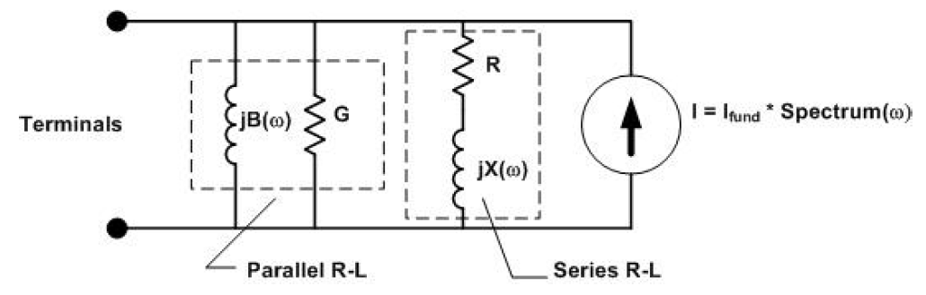
Figure 2. Revised LOAD Model in Harmonics Mode

Users can specify what percentage of the load is to be modeled as a serried R‐L and the remainder will be considered to be a parallel R‐L model. A Property has been added to the LOAD object:

In addition, a global option, NeglectLoadY, has been added that will enable users who so desire to completely neglect the load damping. It is defined as follows:

To use this, you would use the Set command, for example:

Set NeglectLoadY=Yes

Solve ! ‐‐‐ (power flow)

Solve Mode=Harmonics

In January 2015, another option for the defining the shunt admittance of the LOAD model became available. The Series R‐L branch of the model is generally thought to approximately represent the service transformer reactance and other reactances in series with mostly resistive loads. This is what the model would most closely represent if its values are determined from the specified power (kW and kvar) values. The series R‐L branch is also good representation of motors for harmonics studies, but the values would not be determined from the power values. They would be determined by the blocked rotor impedances or subtransient impedances. For a motor, the X would dominate instead of the R.

Therefore, two more properties were added to the LOAD model to force the series branch to more closely model motor and other rotating machine loads: puXharm and XRharm, defined as follows.

By default, puXharm =0, which signifies to the program that the series R‐L branch of the model is to be computed from the power values. If specified as a value >0 it is interpreted as a per unit value on the kVA base of the machine represented by the series branch. If the series branch is set to 50% (the default) that means half of the kVA is assumed to be motor load and that is used as the base to set the value of X in the series branch. The R value in the series branch is then determined by the assumed X/R ratio at fundamental frequency. The typical range for X/R for conventional motors would be

approximately 3‐6. However, some high efficiency motors can have values greater than 10.

This kind of series branch model may reduce some of the lower harmonics because it offers a lower impedance to the injected current, but is highly inductive and tends to block currents from flowing into the shunt path at high frequencies. And because it is inductive, it can cause a shift in system resonances. This is an effect that has been observed in practice and is what inspired the addition of this capability to the LOAD model.

Transformer X/R: XRConst Property

Generally, the resistance in a power system has a minor effect on the flow of harmonic currents when the system is not in resonance. However, the damping of harmonic resonance by resistance of loads, lines, and transformers can have quite a significant impact on the level of harmonic voltage distortion predicted by the models.

Substation transformers and larger transformers supplying industrial consumers have a relatively high X/R ratio of 10 or greater at fundamental power frequency. Distribution service transformers such as those that serve residential loads can have a much lower X/R. It would not be surprising to find that a 25 kVA transformer would have an X/R ratio only slightly greater than 1.0. In either case, there is a question about what to assume for the variation of R for harmonic frequencies.

If no modification to the winding R is made, the equivalent X/R will increase in proportion to the harmonic. This can lead to a prediction of very little damping at harmonic frequencies. For example, if a substation transformer has an X/R ratio of 10 at fundamental, the model will have an X/R of 50 at the 5th harmonic, which generally results in an unrealistically high‐Q circuit model with exaggerated predictions of voltage distortion. The apparent resistance of transformers increases with frequency at a rate that is dependent on its design. The chief component of the increase comes from the stray eddy current losses and can be quite significant in transformers that have conductors with large cross‐sectional areas. Also, designs with conductors in parallel can have circulating currents within the windings that yield an effective increase in R.

Until version 7.6.3 build 13, the OpenDSS transformer model did not have any provisions for modifying R as a function of frequency. The XRCONST Boolean property was added to the TRANSFORMER object. It is defined as follows:

If XRConst=YES the winding R is increased proportional to frequency just like X. This is a typical assumption of harmonics analysts when no other data are available. This approximates what happens in some large power transformers. It will not be a good fit for some transformers, but at least it adds some damping to the model to nullify the exaggerated high voltages and impedances that would otherwise be predicted.

This parameter is not generally as critical for small utility distribution transformers in the frequency range up to the 13th harmonic. The windings are constructed with wire having a small cross section and the stray eddy losses do not generally increase as rapidly as for large power transformers. The normal low X/R of these transformers tends to contribute somewhat to the damping of resonance anyway, yielding results that are only moderately conservative.

Note that the default is NO. Thus, scripts from prior studies will yield the same result when run again.

Future versions of OpenDSS are slated to have user‐defined frequency correction curves. The curves will be applicable to the REACTOR model as well. Until that feature is implemented, if it is necessary to adjust R for frequency, users can script the resistance and solve for each frequency separately rather than using the built‐in Harmonics solution mode or use the REACTOR model to achieve an approximate frequency‐dependent resistance variation.

Figure 3 shows a one‐line diagram of the OpenDSS REACTOR model. The model is nominally a series, multiphase R‐L with user‐defined properties of R and X. In addition to scalar values, R and X may also be defined as matrices. A feature of the model that, perhaps, is seldom used is the parallel resistance, Rp, around the entire branch. Its default value is infinite (open) so that it doesn’t enter into the calculations. However, it can be employed to model frequency dependence of R‐L elements, including transformers. This would require a separate REACTOR to be added in series with the transformer and defined with an appropriate value so that the total through impedance of the transformer is correct.

Figure 3. One‐Line Diagram of REACTOR Object

Comparison of Models

Figure 4 illustrates the different results that can be obtained by the various assumptions about the load damping model.

This figure was created by placing an ISOURCE on the substation bus of a large distribution circuit with 1745 buses and 487 LOAD objects and running several cases varying how the LOAD shunt branch model was created. The harmonic current sources of the LOAD objects were disabled. There are 4 capacitor banks in this model. The ISOURCE was assumed to have a magnitude of 1 A at all frequencies from the fundamental to the 25th harmonic in 5 Hz increments. This type of frequency scan is a common way to characterize the frequency‐response characteristic of a feeder.

The highest and sharpest resonance occurs with no load to damp out the resonance. This model does include the resistances of the lines and transformers. Setting the XRConst=Yes for the substation transformer damps the sharp resonance slightly. The next highest resonance occurs assuming the LOAD objects are represented by a series R‐L derived solely from the specified kW, kvar values.

The characteristic labeled “Default” is 50/50 parallel/series. The magnitudes are between the All Series RL model and the All Parallel RL model as expected. The All Parallel RL model yields the most damping. If we take the Default model and declare that the series part is motor load with a fundamental frequency reactance of 0.20 pu, we see the characteristic shift to the right (higher frequency) on the diagram. This makes sense because adding 487 small susceptances in parallel with the substation will reduce the net apparent reactance involved in the resonance, increasing the resonant frequency from approximately the 10th harmonic to the 12th harmonic.

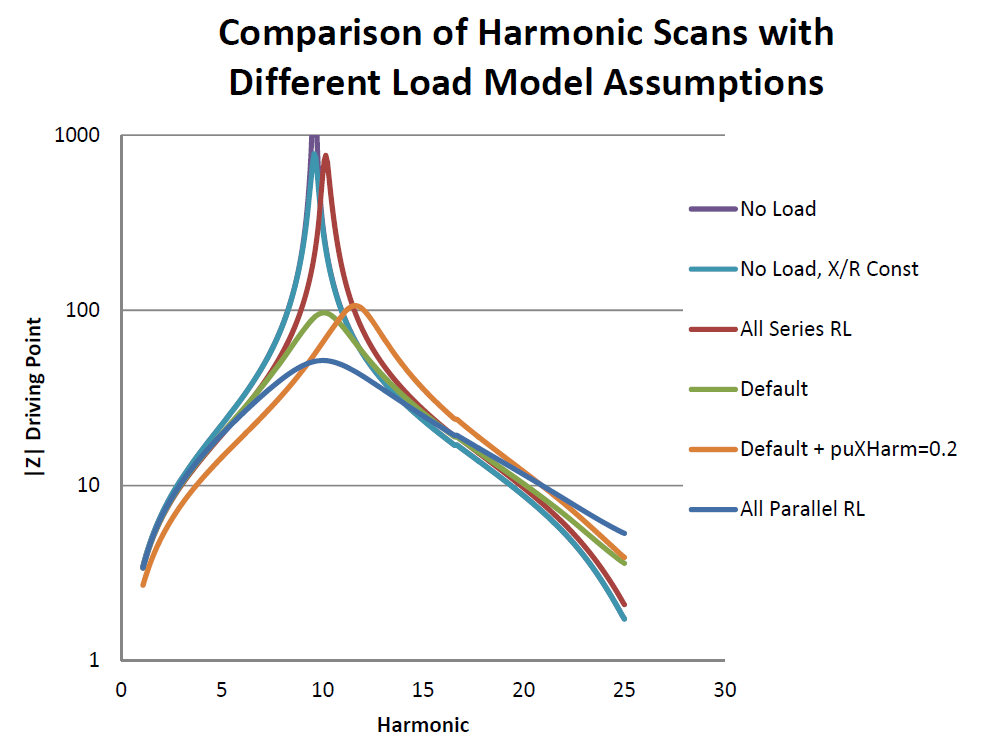
Figure 4. Comparison of Effect of Using Different Load Models

Figure 5 shows another comparison of the impact of the different LOAD object models. This represents

the harmonic distortion solution for bus 82 in the 123‐bus test feeder. It was obtained by doing:

1. A power flow solution at the given load level (Solve in Snapshot mode)

2. Solve Mode=Harmonics

The LOAD objects at non‐fundamental frequencies are converted to current sources using the DefaultLoad harmonic SPECTRUM object. Thus, OpenDSS solves at harmonics 3, 5, 7, 9, 11, and 13. The results for the different ways of modeling the shunt admittance branch of the LOAD objects are displayed on the figure.

The highest distortion is predicted when the shunt admittance branch is neglected (Set NeglectY=yes). This would be the expected result. However, the 7th harmonic voltage is predicted to be higher for both the All Series and Default + Motor cases. The IEEE 123‐Bus Test Feeder has resonances near the 5th and 7th harmonics. It is interesting to note that at frequencies where the system is not resonant, the results are not particularly sensitive to the model of the shunt admittance. It is only at frequencies near the resonances that there are significant differences.

If we ignore the NeglectY=yes case, the predicted harmonic voltages differ by less than a factor of 2. Because THD is computed by square root of sum of squares, there will generally be even less difference in the THD values. Interestingly, the default 50/50 model comes in about average for all cases and this suggests it should be a good guess when nothing else is known. Employing the newly‐added capability to better represent motor loads shifts the system resonance slightly higher, which results in the 5th harmonic to be lower and the 7th harmonic to be higher. The main factors in determining the distortion are the characteristics of the feeder lines, substation transformer, and capacitor banks.

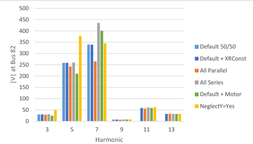
Figure 5. Harmonic Distortion Solution for IEEE 123‐Bus Test Feeder