Load Models That Nearly Always Converge
One problem with nearly all power flow solution algorithms is that it is difficult to maintain a converged solution over a wide range of voltages. OpenDSS is no exception to this, but the load models have been modified so that they nearly always converge for very low voltages. The modification is illustrated in Figure 1.
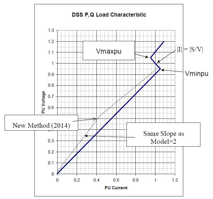
Figure 1. Load Model Modification to Maintain Power Flow Convergence.
This is illustrated for the common constant power load model (OpenDSS Model=1, the default). The problem is the hyperbolic characteristic between Vmaxpu and Vminpu voltages. As the voltage continues to drop, the current increases significantly if it is assumed that S remains constant. When the voltage drops to about 70%, or below, the iterative solution often fails. Some analysts assume that when the power flow fails to converge, that will also happen on the actual power system. This is more true of the transmission grid than the distribution system. The voltage collapsing on the distribution feeder generally does not cause voltage collapse on the bulk power supply.
The voltage will sag low, but the system will generally continue to function in some regard and will recover to normal voltage when the fault causing the sag is removed. The actual voltage can be anything between 0 and normal voltage and EPRI has thousands of power quality voltage sag measurements to prove it.
Also, for multiyear planning studies the voltage will sag low as the load grows year after year. Users do not want a 20-year 8760-hour yearly simulation to bomb out 12 years into the simulation. Such simulations can take hours and you want to avoid having to repeat a simulation simply because the voltage went low. It is sufficient to know that the voltage is low in some hours and planners will have to fix something.
The OpenDSS solution is to revert to a linear model when the voltage drops below the value specified by the VminPU property of the Load model. The load characteristic shifts to a straight line from the VminPU point to zero. This proved adequate for several years, but is not a perfect linear impedance model that would always converge.
It was known that loads modeled as Model=2 (constant impedance) always reached a converged solution. As shown in Figure 18, a further modification was made in 2014 to transition the slope of the linearized model to exactly what a Model=2 load would have at some lower voltage point. A new Load model property was introduced, named VlowPU, to define the breakpoint for this transition. This value defaults to 50% and should not be set much different than this.
With the modified linear model, you can actually place a Fault object on the circuit while performing a power flow and it will converge most of the time. Will the answer be accurate? That all depends on your model. It is probably not very accurate if there were meters on the system to show the actual value, but simply indicating a low voltage is sufficient knowledge for planners. The key is that the program will generally not break and your simulation can proceed.