Putting it all Together
This section s dedicated to describe the power flow solution methods implemented in OpenDSS. OpenDSS uses three solution methods for solving the power flow problem:
set algorithm=Normal
set algorithm=Newton
set algorithm=NCIM
Figure 1 depicts the general solution algorithm in which the power flow solution goes first, and then the control actions to operate over the latest solution found.
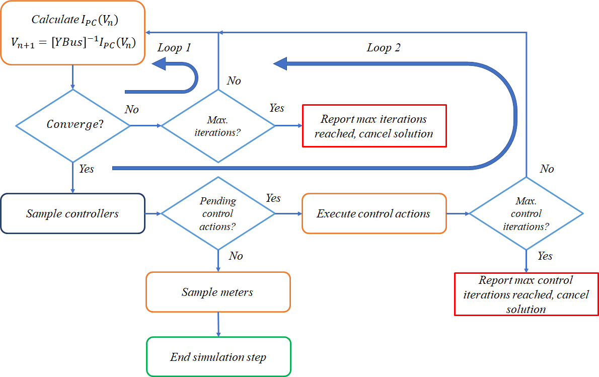
Figure 1
Solution algorithm in OpenDSS