OpenDSS Documentation

Modeling Transformer Core Effects in OpenDSS

BackGround

For distribution system analysis studies that involve only power flow analysis, it is generally sufficient to model 3-phase transformers using the positive-sequence leakage impedance parameters. You rarely need to represent the magnetizing impedance unless you are doing loss analysis that is sensitive to the magnetizing current. However, there are types of analysis where the zero-sequence response of some types of transformers is important to model. Since the OpenDSS models transformers as they are physically rather than using symmetrical component equivalents, you have to understand a little more about transformer behavior than you might otherwise.

The main issue is with transformer core structure of 3-phase transformers. The existing OpenDSS Transformer model does not represent the transformer core other than as a linear reactance (if the “%imag” property is greater than zero). The magnetizing branch is embedded within the matrices as the impedance matrix is computed. Therefore, it is difficult to separate it explicitly from the model. Most of the time, this is sufficient for distribution system analysis, but there are exceptions. One, in particular, is when the characteristics of the magnetic circuit in 3-legged core transformers results in significant impacts on zero-sequence impedances. The present Transformer model in OpenDSS assumes no magnetic coupling between the phases. Coupling between phases is accomplished by electrical connections of the windings. So when it becomes important to model the core effects on the zero sequence impedances, something special must be done.

Instances Where Modeling 3-Legged Core Effects Might Be Important

• Manufacturers have told me that the vast majority (>90%) of the utility distribution substation transformers are core-type transformers (3-legged core designs – sometimes called “E” cores). Thus, the single-phase fault current at the primary distribution bus can be slightly higher than what one might get by assuming the zero sequence leakage impedance of the transformer is the same as the positive-sequence leakage impedance. Whether this is important depends on the purpose of the analysis. If you are most interested in things that happen more than ½ mile or so out on the feeder, it generally doesn’t matter much. However, if breaker duties due to DG infeed are being computed at the substation bus, it could be important.

• Many of the distribution substation transformers in areas where the transmission system is strong are two-winding transformers connected Delta-Yg. It is typically most important for these transformers for the zero-sequence model to be correct only when looking into the Yg side. The physical Delta winding dominates the effect while the core model makes a minor contribution to the zero sequence. However, in many other systems such as where the transmission system needs a lower grounding impedance, the distribution substation transformers are 3-winding transformers connected Yg-Delta-Yg. The delta winding (usually called the “tertiary” winding) is frequently unloaded and buried, but in some cases reactors or capacitors may be connected to it to support transmission functions. For many distribution system analysis cases, it is only necessary for the transformer model to appear accurate from the distribution side of the substation. However, the OpenDSS can represent the transmission system simultaneously and it may be important for the transformer model to be accurate when looking from both transmission and distribution sides of the substation.

• Most utility 3-phase distribution (service) transformers these days are made up of either a bank of single-phase transformers or are 5-legged core padmounted transformers. Nothing special needs to be done for these transformer designs for the typical kinds of studies that OpenDSS can perform. Simply define the transformer using the high-to-low leakage impedance from the test report or nameplate. A special 5-legged core model may be important for time-domain (i.e., EMTP) studies such as ferroresonance, but rarely for OpenDSS studies. On the other hand, I have encountered many 3-legged core dry-type service transformers connected at primary distribution voltage levels. Some are owned by utilities, but the majority were installed by end users. It usually doesn’t matter significantly for power flow calculations, but these transformers can have an impact on the single-phase fault current calculations and on any condition where one phase is open or is otherwise grossly unbalanced. The latter is often quite important when considering things that can go wrong with DG installations. The common Yg-Yg transformer connection on a 3-legged core will behave as if it has a 3rd delta-connected winding (called a “phantom” tertiary), which can lead to surprising results.

Symmetrical Components and the OpenDSS Program

Many power engineers are accustomed to have fault current calculation tools that form positive-, negative-, and zero-sequence networks and connect them in various ways to compute fault currents and other quantities resulting from significant unbalances. Unfortunately, in order to meet its analysis and modeling objectives, the OpenDSS cannot use this approach. There are many system conditions such as unbalanced lines that cannot be accurately studied with symmetrical component models – at least not easily. Network unbalances result in coupling between the sequence networks. When the networks end up coupled together, it is usually simpler to solve the system in phase components, which is the OpenDSS approach. Also, the OpenDSS is capable of n-phase models, not just 3-phase models. Symmetrical component transformations technically do not apply to circuits with other than 3 phases (either more or less). For 1- and 2-phase models, there are certain kluges1 that power engineers have applied that give approximate answers.

Per unit representations raise another issue. Per unit models were introduced into power system simulation to be able to model multiple voltage levels without having to specifically represent the transformer. The OpenDSS is capable of analyzing problems where impedances span transformers, which are difficult to represent in per unit systems without resorting to kluges. Two common examples are:

1. High-to-low capacitance in transformers for certain harmonics problems, and

2. The 69 kV overbuild falling into the 12.5 kV distribution line.

Also, the common split-phase 120/240V residential service transformer is not amenable to per unit representation when there are both 120V and 240V loads. Which base do you use?

Therefore, the OpenDSS represents everything in admittance matrices in units of actual Siemens. Voltages and currents are likewise in units of actual volts and amperes. While 30 years ago this frequently resulted in a problem with numerical accuracy because of the great differences in the numerical values at different voltage levels, modern numerical methods with at least 64-bit floating-point arithmetic pretty much makes this a non-issue. There are few distribution system circuit modeling conditions in which the equations are sufficiently ill-conditioned to require remedial actions.

Both of the issues in the preceding paragraphs have a bearing on the transformer model in the OpenDSS. As a Power Delivery element, a transformer is ultimately modeled by a primitive Y matrix that embodies all impedances and winding connections. No attempt is made to model the nonlinear portion of the magnetizing impedance within the transformer model; it is modeled as a linear reactance, if specified at all - %imag defaults to zero. The model is focused on the leakage impedance behavior, which has the most impact on power flow, harmonics, etc.

The OpenDSS transformer model, like other models in OpenDSS, is a physically-based model. Windings are modeled and connected as they would be in the actual transformer. A split-phase service transformer is actually constructed as a 3-winding transformer and must be modeled that way if necessary to capture the true behavior. In some analysis programs, one might represent a phase shifting transformer by specifying the phase angle. In the OpenDSS, you would define and connect the windings as the manufacturer would when the phase shifter is built. With this is mind, let’s go back to the 3-legged core transformer model.

Figure 1 shows the schematic for a Yg-Delta-Yg transformer. If this transformer is constructed from three single-phase transformers, a shell-type 3-phase transformer, or even a 5-legged core 3-phase transformer, we generally do not worry about interphase coupling of the magnetic circuit for the types of analysis performed with OpenDSS. Of course, the delta winding provides coupling between the phases.

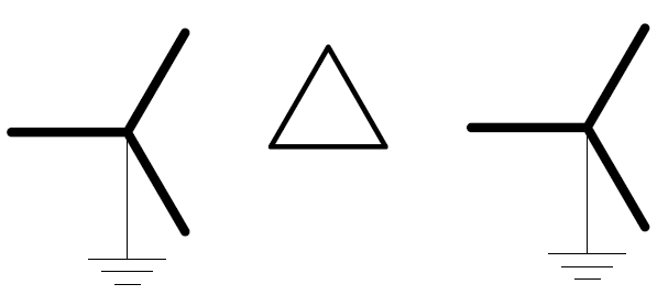
Figure 1. Yg-Delta-Yg Transformer

There are 3 short circuit measurements between each pair of windings required to construct the short circuit reactance matrix as depicted in Figure 2. The OpenDSS can take this matrix and construct a full 12x12 primitive Y matrix that represents the transformer windings including the neutral point.2 (A dummy neutral point is generated for the delta winding to satisfy an OpenDSS requirement that all terminals have the same number of conductors. By default, it gets connected to ground and its current is zero.)

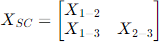
Figure 2. Short circuit reactance matrix required to represent a 3-winding transformer (percent or per unit values).

The OpenDSS transformer model provides the XHL, XHT, and XLT properties as a means for specifying the reactances of a 3-winding transformer. Alternatively, users may use the xscarray property, which accepts the short circuit reactances as an array representing the lower triangle matrix depicted in Figure 2.

Note that some data sources provide per unit or percent values for XH, XL, and XT to represent a 3-winding transformer (Figure 3). Keep in mind these values are for a model that works for the special case of a 3-winding transformer. In reality, there are no corresponding physical values for these reactances. A clue to this is that XL frequently comes out negative.

Figure 3. Three-branch per unit or percent model commonly used in power system analysis programs.

The reactances arise from the leakage flux between pairs of windings. OpenDSS is designed to model transformers of nearly arbitrary numbers of windings. All that is required to construct the model are short circuit impedances between each pair of windings. Very complex models can be constructed in this way depending on the ability to compute or measure the short circuit impedances.

Phantom Windings

If the transformer is constructed around a 3-legged core, there is a complication to specifying the short circuit impedances between the windings. As shown in Figure 4, zero sequence flux is in phase in each leg of the core and has to leave the core to complete the magnetic circuit. The path is mostly “air core” (i.e., not in steel). Thus, the magnetizing reactance to zero-sequence flux is considerably less than for other normal mode fluxes (positive- and negative- sequence, for example). In fact, although it is larger, it is of the same order of magnitude as the leakage (short circuit) reactances and often cannot be neglected.

The net effect for a 3-winding 3-phase transformer is like having separate cores for each phase but having a 4th delta-connected winding. In transformer literature, this is often referred to as a “phantom” delta winding as depicted in Figure 5. A 4-winding model is required to construct a physically-based model of the Yg-Delta-Yg transformer if we choose not to neglect the error introduced by neglecting, or approximating, the phantom winding effect. Unfortunately, the phantom winding does not physically exist and a measurement of the short circuit impedances cannot be made. Measurements can be made only to the physical windings. However, some transformer design programs can compute these values (I used to work for a transformer manufacturer and could obtain the appropriate values from the Engineering Department on special occasions).

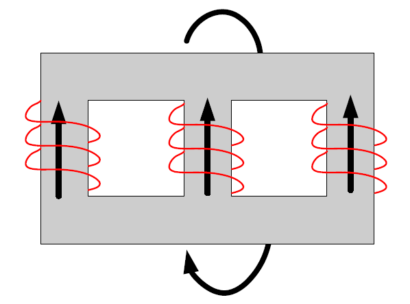
Figure 4. Three-legged core zero sequence flux paths.

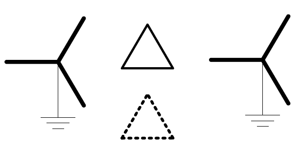
Figure 5. The effect of the 3-legged core is like having an extra "phantom" delta-connected winding

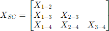
Figure 6. Ideally, one would provide three additional short circuit measurements to the phantom winding.

Modeling Options

Having a physical delta winding on the core will help with zero-sequence modeling. It will naturally get the zero-sequence impedance in the ballpark of where it should be. But the zero-sequence impedance still needs to be a little lower. Options for OpenDSS modelers include:

• Define a 4 winding transformer in OpenDSS and estimate the 3 additional short circuit measurements. Sometimes, these can be reasonably estimated from transformer test reports, but not always. For modeling a 2-winding transformer on a 3-legged core with this approach, you would define a 3-winding transformer and estimate values for the XHT and XLT properties.

• If the physical delta winding is not to be loaded, one option is to define a 3-winding transformer and reduce the values of XHT and XLT to more closely match the zero-sequence short circuit measurements. XHL is specified as the positive sequence value so that the basic power flow solution is correct. This approximation is good enough for many studies.

• The transformer is defined as a 3-winding transformer and the positive-sequence leakage impedance values are used for the XHL, XHT, and XLT properties. Then add a separate Yg-Delta 2-winding transformer on the Low voltage Yg winding with an appropriate impedance to bring the net zero-sequence impedance down closer to the tested value. The additional transformer acts as a grounding transformer. You could also define a zig-zag transformer, but a 2-winding transformer is much easier in the OpenDSS. Again, this approximation is satisfactory for many studies involving the distribution feeder. It may not be good enough if impacts on the transmission system are critical.

• The OpenDSS allows another modeling option not available in other programs. You can define the transformer model using the zero-sequence model values and then add a special positive sequence impedance in series with the High winding of the transformer to make up the additional impedance seen by positive- and negative-sequence currents.

Estimating Impedances to the Phantom Winding

For the case where you choose to estimate the impedance to the phantom delta winding, the values of the short circuit reactance from the actual winding to the phantom winding are typically in the range of 75 – 200 % on the main transformer’s kVA base. In parallel with the physical Delta, for which the reactances are typically in the 7 – 30% range, this reduces the net zero sequence impedance by 5-10% from the positive-sequence impedance. To better understand what values to choose, it is necessary to understand more about how transformers are constructed.

As shown in Figure 7, the physical Tertiary winding is generally wound next to the core. Then the Low voltage winding and the High voltage winding are wound on top of the Tertiary in that order. The short circuit reactance is proportional to the physical space between the winding. The greater the space, the higher the reactance is. Proportions vary with designs. The default values in the OpenDSS transformer model are XHL=7%, XHT=35% and XLT = 30%. The Low winding is closer to the Tertiary than the High winding. Thus, XLT is lower than XHT. In another transformer (from the example in this document) in which the Low is physically much closer to the Tertiary the values are XHL = 8.98%, XLT = 7.3%, and XHT=13.32%.

For estimating the short circuit reactance to the phantom winding, we need to come up with three values as indicated in Figure 6. One might think of the phantom (4th) winding as occupying the space inside the Tertiary winding. The Tertiary (3rd) winding is closest, so X3-4 would be smallest of the three and X1-4 (High to phantom) would be the largest. Knowing these proportions, we can make some educated guesses and can generally match test results after a few quick iterations using OpenDSS scripts.

Figure 7. Typical coil arrangement for a 3-winding transformer.

Adding a Positive-sequence Reactor to In Series with the Transformer

The basic idea here is to define the transformer using the zero-sequence impedances and add a little impedance in series with the High winding to make up the difference between the zero-sequence and positive-sequence impedances. The trick is that the added impedance appear only in the positive-sequence network.

The same principle applies to 2-winding transformers on a 3-legged core. The problem is not as complicated for a Delta-Yg substation transformer common in many areas, so it is a little easier to comprehend. Here is one procedure:

1. Define XHL = the zero sequence value measured from the Yg side, if this information is available (unfortunately, it is not always readily available; the positive-sequence impedance is often the only one supplied for a two-winding transformer). This value is used because it is the smaller reactance of the positive- and zero-sequence reactances.

2. Add a reactor on the Delta side with a reactance value equal to the difference between positive- and zero- sequence impedance. Alternatively, the difference can be embedded in the source equivalent in some cases. (Don’t forget to convert to ohms on the Delta winding voltage base.)

This procedure works well for a 2-winding Delta-Yg transformer because the delta winding prevents the flow of zero-sequence currents into the High side. Therefore, any reactance added to the high side responds only to positive- and negative-sequence currents. This will NOT work for a Yg-Delta-Yg 3-winding connection. This connection will allow zero-sequence currents to flow in the added reactor and will have an impact on the zero-sequence equivalent.

Fortunately, the OpenDSS allows for a workaround. Many elements, including the Reactor object can be defined with a matrix. This allows one to define all sorts of strange impedance characteristics, including some that may not be physically realizable. If you define the reactance matrix with values in the ratio shown below, the Reactor will have only positive-sequence impedance and the impedance to zero-sequence currents will be zero.

The self (diagonal) term is

Zs = 1/3 [ 2Z1 + Z0 ]

The off-diagonal value is

Zm = 1/3 [ Z0 – Z1 ]

Setting Z0 = 0 yields the values to use for the R and X matrices.

The only problem with this approach is that matrices of this precise form are singular and cannot be inverted (they need to be inverted to be changed into admittance form). However, I have found that if you create a little imprecision in the R matrix – so that R0 is not precisely 0 – the Z = [R +jX] matrix inverts quite nicely in the OpenDSS. In the second example below, the Rm value was rounded up in the 5th decimal place and it worked OK.

Examples

Two examples of modeling a 3-winding Y-D-Y 30 MVA transformer to meet the following impedances:

Positive sequence: 10.79%

Zero Sequence:

XHL = 8.98%

XLT = 7.3%

XHT=13.32%

Both models use a bank constructed of 1-phase units for clarity, although a 3-phase model could also be used.

Estimating Impedances to 4th (Phantom) Winding

In this case, the base 4-winding model is built using the positive-sequence short circuit reactances. Then the impedances to the phantom (4th) winding are adjusted until the SLG fault currents match the test results. Knowing the typical values were in the 75% to 200% range, I started by guessing

X1-4 = 100%

X2-4 = 80%

X3-4 = 75%

This was based on my assumption of the construction of the windings (see above). This turned out to be a good guess because I had only to drop the last two values slightly to obtain the desired fault currents.

X1-4 = 100%

X2-4 = 70%

X3-4 = 65%

This took only 4 or 5 iterations using the script on the next page. Note that this script uses the new XfmrCode object to define the transformer. If you get an error when you run this, you will need to update your version of the OpenDSS.

Figure 8. Model with three 1-phase 4-winding transformers

Adding Positive-Sequence Only Reactance

In this method the base 3-winding transformer is defined using the zero-sequence impedance values. Then a Reactor element is added in series with winding 1 to make up the difference so that the positive sequence model matches test results. Note that the off-diagonal elements of the Rmatrix are rounded up to create a little imprecision so that the Reactor’s Z matrix can be inverted. The Reactor values are in ohms at 161 kV.

Figure 9. Model with three 1-phase 3-winding transformers and an added Reactor

Using Transformers To Help Model A Generator

We often use similar concepts, depicted in Figure 10, when modeling synchronous generators in which X0 is much smaller than either Xd’ or Xd”. The present Generator model does not support the specification of X0 separately. So we add a transformer in front of the generator to obtain the proper X0. Without this model, the Generator primitive Y matrix would result in X0 = Xd’ or Xd”, whichever is being used for analysis at the moment. This general form of the model would be mainly needed for dynamics, short circuit, or harmonics studies of synchronous generators directly connected to the utility distribution studies. However, we have also found that it often has superior convergence characteristics for power flow studies in which convergence is more difficult than normal.

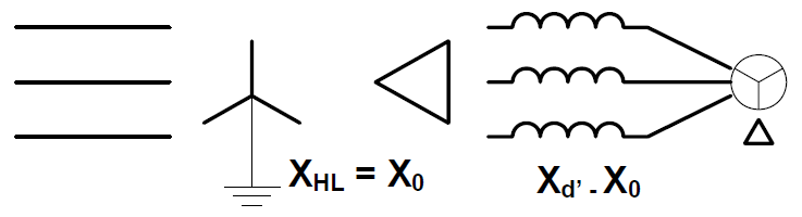
Figure 10. Using a Yg-Delta transformer to help model a synchronous generator for short circuit studies.

The impedance of the Yg-Delta transformer is set to X0, which is the smallest impedance. The generator is defined as connected in Delta with an impedance equal to the remainder of the Xd’ impedance (for harmonics studies, you would use Xd”). If the transformer is defined with the same kVA rating as the generator, no conversion of the impedance values is needed. However, note that the Transformer model reactances are in percent and the Generator model reactances are in per unit. Thus, looking from the Y side of the transformer, the total model has the desired impedance characteristics.

If there is an interconnection transformer, the impedances of the transformer can be combined with X0 of the generator. If the interconnection transformer is Delta-Y or Delta-Delta, the disposition of X0 is probably of little consequence. Note that if the interconnection transformer is Yg-Yg (as is common in some areas) and the generator is grounded at the neutral, it is still preferred to model the generator using the connection shown in Figure 10 with the impedances adjusted accordingly. Two separate transformers can be used, or combined into one.

When modeling a Y-connected generator with a significant neutral impedance, the power flow solution will almost always converge better if the Generator object is defined as connected in Delta and is fronted by a Yg-Delta transformer as shown. The neutral impedance would be a separate Reactor element placed in the neutral of the Transformer object Y winding. Otherwise, you will probably have to relax the convergence criterion to 0.001 or higher to allow the generator neutral to wobble around a little as it seeks convergence.