Modeling Multi-Winding Transformers
Modeling Multi-Winding Transformers
Figure 1 shows the common 3-winding transformer equivalent model used in power system analysis based on positive-sequence equivalent circuits. This is used in nearly all (if not all) of the popular transmission system power flow, short-circuit, and dynamics tools. The popularity of the model likely stems from the fact that it can be constructed entirely from simple two-terminal R-L branch models. This makes the programming somewhat simpler, although it does create some issues because a single device (a transformer) is modeled by three branches. So programs usually contain some “kluge code” to keep track of branches that are associated with transformers. Also, it requires the creation of a fictitious node (M) that doesn’t physically exist.
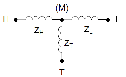
Figure 1. Common Model of 3-Winding Transformers used in Positive-Sequence Analysis
This model is so ingrained in the minds of electric power systems analysts that many, if not most, think the impedances in the model are actually found somewhere in a transformer. It is not until one encounters an unusual transformer such as a 4-winding transformer that one discovers that this modeling approach works only for the special case of a 3-winding transformer.
The leakage impedance network of a 3-winding transformer is defined by (3x2)/2 = 3 short circuit tests that yield ZHL, ZHT, and ZLT. The formula for the number of short circuit tests required is: N(N-1)/2 where is N is the number of windings. A model need 3 degrees of freedom to model a 3-winding transformer.
The model in Figure 1 has 3 degrees of freedom, so it works. A 4-winding transformer is defined by (4x3)/2 = 6 short circuit tests and requires 6 degrees of freedom. Some sort of mesh circuit is required to represent the transformer leakage impedance characteristic. It may be impossible to create a star model that is accurate. The same can be done for the 3- winding case. The model in Figure 2 can be made equivalent to the one in Figure 1 and does not require the creation of a fictitious node. Note: ZH-L is not the same as the shortcircuit impedance between H an L, ZHL, above; it can be obtained by a simple star-delta conversion from the circuit in Figure 1. Inside a power flow program, a Kron reduction can be performed on the admittance matrix to eliminate the fictitious node. This will accomplish the same thing as the star-delta conversion.
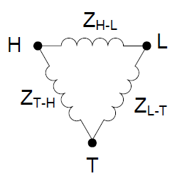
Figure 2. Equivalent Model that Does Not require Fictitious Node
The architects of the Common Information Model (CIM) chose to use the values of ZH, ZL, and ZT to describe a 3-winding transformer. Each winding – H, L, and T – of the transformer is stored in the database separately, each with a single value of resistance, R, and reactance, X. While it might be argued that it is acceptable to store the resistance with the winding model because each winding does indeed have resistance, there is no such thing as the reactance of a single winding, such as XH, for example. Short-circuit leakage reactances only exist between pairs of windings. If the architects of the CIM had wanted to model transformers more correctly, they would have defined a separate object to contain short circuit tests, of which there would be 3 for a 3-winding transformer. This defect (in my opinion) in the CIM has caused problems trying to adapt it to distribution system analysis, which uses more complicated transformer models. As it is, one can only model 2- and 3-winding transformers.
Reasons for NOT using the model in Figure 1
• The model requires the creation of an additional node.
• Need to model a transformer with more than 3 windings.
• XL often comes out negative for autotransformers with tertiaries.
• It is incapable of modeling the most common 3-winding transformer in the North American power grid – the ubiquitous split-phase distribution transformer.
Each of these points is addressed further in the following:
Each fictitious node requires an equation in a nodal admittance formulation. In a case with hundreds of transformers, this could add significant time to the solution. So it would be nice to avoid this with a model that does not require an extra node. In the case of a three-phase model, the impact of the extra nodes could be even greater than for a simple positive-sequence model.
While not common in the transmission grid, transformers with more than 3 windings show up in various industrial processes and have also been used to connect inverter-based DG such as fuel cells. They are used to provide isolation between devices with electronic power converters.
A negative XL is not necessarily a show stopper. If it can be buried in the system Y matrix along with overwhelming positive values of the other parts of the model, it is seldom a problem. It was a problem in the past with models in electromagnetic transient analysis where the integration formulae would yield unstable solutions for a R-L branch defined with negative inductance. It used to be common to ignore the small negative XL branch to avoid this. It is not known whether this is still an issue, but I suspect most transients program vendors use more sophisticated transformer models now. But this is something to keep in mind if creating software for transients analysis.
While it is common to think of a residential service transformer only as a simple single-phase 2-winding transformer, it is actually a 3-winding transformer. It has one primary-voltage winding and two 120-V secondary windings. While it might seem like it is just like the single-phase model used in a positive-sequence power flow, it is not. In the transmission model, the three windings are connected to the power system model with the same polarity. In the distribution transformer model, the two secondaries are connected in series. The grounded terminals of the secondaries are connected in opposite polarity. The link below describes how the transformer is modeled in OpenDSS
To make the modeling problem for the distribution transformer more interesting, the mixture of 240 V and 120 V loads makes it impossible to model the transformer with a single per-unit model. (Try it if you don’t believe me.) That is one reason why we don’t use per-unit models of lines and transformers in the distribution analysis tools such as OpenDSS. A more general transformer model is needed.
A more general way to model transformers
Is there a way to avoid these issues? Let’s take a look at a general method that will allow the construction of a leakage impedance model of nearly any transformer for power system analysis.
While I learned the conventional 3-winding model for power flow in college and have worked with several computer programs that use it, I learned a different way of modeling transformers in 1973 and have used it almost exclusively in programs I designed and wrote myself. At the core of most power systems analysis programs whether for power flow, short circuit, harmonics, dynamics, or transients, is a system nodal admittance (Y) matrix. Y may be a plain nodal admittance matrix, an augmented matrix or a component of another set of equations such as a Jacobian for a Newton-based solution. The general approach is to first build Y from so-called “primitive” admittance matrices for each element.
For the simple 3-winding transformer in Figure 1, a primitive Y matrix, YPrim, is illustrated in Eq. (1).
 (1)
(1)
This equation relates the transformer’s terminal currents to the node-to-ground voltage at the terminal. This is the voltage of the positive-sequence network model. Thus, every element of YPrim can be summed directly into the system Y matrix. There is a direct mapping of each element of the YPrim matrix to the system Y determined by a terminal-tonode incidence list.
The YPrim matrix can be constructed directly from short-circuit test data. There is no need to generate an intermediate equivalent circuit. This method applies not only to a simple single-phase positive-sequence model but to general n-phase, m-winding transformers. This is the approach used in OpenDSS.
Here is description of the method adapted from my paper with Surya Santoso presented at the 2003 IEEE T&D show: (Note: Equation numbering restarts at 1.)
--------------------------------------------- Insert ----------------------------------------------------
The Transformer Model
Some of the methods for modeling transformers use the per unit system and some use actual values. The authors prefer to work in actual values and will demonstrate that method here. The objective of the method described here is to develop a “primitive” nodal admittance matrix, Yprim, describing the transformer. Once the transformer impedance model is in this form, it can generally be incorporated quite easily into most system solution algorithms.
The method permits the modeling of the leakage impedance network of any transformer with any number of phases and any number of windings connected in an arbitrary fashion. It works equally well for developing inductance models for time domain analysis, where it is perhaps more commonly employed, or models of complex impedance values for steady state analysis. The latter is more applicable to distribution system analysis. Therefore, the notation will be presented in terms of complex impedance (z) and admittance (y) values. Bold uppercase letters designate matrices or vectors while lowercase letters designate scalar values.
The starting ingredients are:
1. The short circuit impedance between each pair of windings,
2. The turns ratio or voltage ratings of the windings.
One of the reasons we have adopted this approach is that transformer manufacturers can generally provide accurate values for the short circuit impedances between windings by test or empirical formulae for any number of windings.
From these data, the short circuit impedance matrix, ZB, is constructed with one of the windings serving as the reference (assumed shorted). The process is identical to forming the short circuit matrix for a power system with the infinite bus as reference. Thus, the designation, ZB, is borrowed from that area of power system analysis.
The short circuit impedance between windings i and j, which we will designate zSCi,j, is generally expressed in percent on some voltampere (VA) base, usually that of the first winding. Let zbase be the multiplier to convert to a convenient voltage base. We generally use either a one-turn or a one-volt
depending on how the turns ratios are to be expressed (turns or voltages). This is an arbitrary choice that is simply a matter of choosing the appropriate multiplying factors and any base will work.
With the first winding as the reference winding, ZB is constructed as follows:
Diagonal Elements of ZB
ZBii = zSC 1, i+1 x zbase for i = 1 to m-1 (1)
where m = number of windings.
Off-diagonal Elements of ZB:
ZBij = 0.5[zBii + zBjj - zScj+1,i+1 x zbase] i ≠ j (2)
Note that the order of ZB is (m-1) – one less than the number of windings. For a simple 2-winding, single-phase transformer, ZB is trivial, having only one element.
Once this matrix is computed, any arbitrary transformer connection may be modeled by simply applying linear algebra to perform power-invariant reference frame changes and the conversion to actual values. The desired result here is the primitive admittance matrix for the transformer. This is merged with the primitive admittance matrices for other elements in the system to form a system nodal admittance matrix, Y, representing the connections to the buses in the system. Therefore, the immediate goal is to transform ZB into the corresponding primitive admittance matrix, Yprim. The transformation can be written in matrix notation as shown in Equation (3).
B is defined as an m x (m-1) incidence matrix whose elements are either 1, -1, or 0. It relates currents in the short circuit reference frame where the first winding is assumed shorted to the currents in the nodal admittance reference frame on a one-turn or one-volt base designated Y1. This network is essentially a perunit value model with no winding connections represented, similar to what one might use for a positive-sequence power flow.
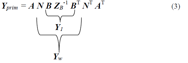
N is either a m x m or a 2m x m incidence matrix whose non-zero elements are the inverse of the number of turns in the windings (or the voltage rating of the winding, depending on the base of ZB). The matrix is 2m x m if you wish to explicitly represent each terminal of each winding individually at this point. This matrix relates the currents in the Y1 equation to the actual winding currents. The resulting admittance matrix in the winding reference frame, YW, is in actual values (S). The voltages and currents in this reference frame are the voltages across the windings and the currents through the windings.
The A matrix is an incidence matrix, whose non-zero elements are generally either 1 or -1, that relates the winding currents to the actual transformer terminal currents. A single-phase, two-winding transformer would yield a 4x4 Yprim matrix because there are 4 conductors available for connecting to something (two conductors per winding). A three-phase, wye-delta transformer with the neutral terminal explicitly modeled would yield a 7x7 Yprim matrix. (In OpenDSS it would be a 8x8 because all terminals must have the same number of conductors and there is a neutral conductor for the delta winding that is not connected to anything.)
Note that nowhere in this formulation is a three-phase system assumed. There are not necessarily any values appearing in the incidence matrices as in many formulations found in the literature. When the  is used, the model generally applies only to 3-phase transformers. The model described here will work for any number of windings and phases. The phases do not have to be balanced nor must they have the same turns ratios. If you get the short circuit impedances, number of turns, and the winding connections correct, everything will come out correctly in the system model. Whether the transformer is single-phase, threephase, or n-phase unit, the notation stays the same. Only the contents of the matrices are changed.
Figure 3 illustrates the process defined in Eq. (3) schematically.
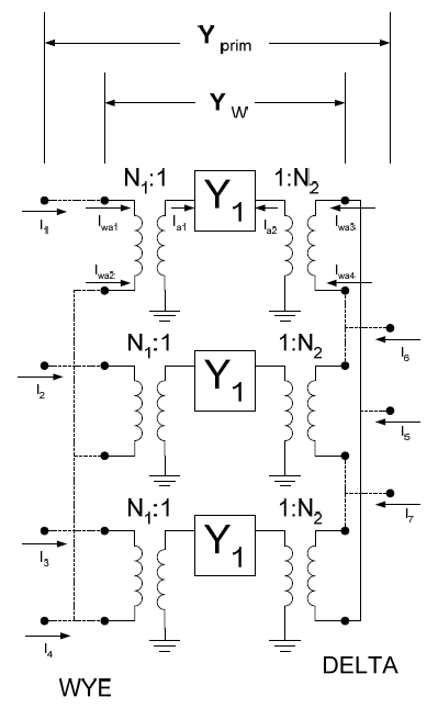
Figure 3.Schematic of transformer model development for a simple wye-delta 3-phase transformer.
Y1 represents a ground-referenced nodal admittance network that will give the proper leakage impedance model on a one-turn or one-volt base. The N matrix represents the effect of the ideal transformers shown to obtain actual winding voltages. Finally, the A matrix represents the connections of the winding conductors to obtain the transformer terminals as depicted by the dashed lines. A neutral impedance of wye-connected windings can be implicitly included in Yprim by adding the appropriate admittance to the corresponding diagonal element (Yprim 44 in this case).