TechNote AutoAdd Solution Mode
The “Autoadd” feature is a mode in OpenDSS that the user can use to study the optimal placement of distributed generation or capacitors. Either capacitor or generator optimization can be studied by defining the “Addtype” option.
The default “Addtype” is generator. The result of adding generators is displayed most effectively as a “daisy” plot on the graphical representation of the circuit. The results of the daisy plot help indicate places where the feeder needs to be strengthened.
In the example script below, the mode is set to “AutoAdd”. The generator power of each generator to be added is set to 100kW at unity power factor. The program searches each available bus for a location that gives the greatest per unit improvement in a combination of losses and capacity. You can use the Set AutoBusList option to limit the buses to be checked. You can define this option by an array of bus names or you can specify a text file holding the names, one to a line, by using the syntax (file=Myfilename.txt) instead of the actual array elements (just like other DSS array properties). Default is null, which results in the program using either only buses in EnergyMeter object zones or, if no EnergyMeters, all the buses, which can sometimes make for lengthy solution times.
Examples:
Set autobuslist=(bus1, bus2, bus3, ... )
Set autobuslist=(file=buslist.txt)
The AutoAdd feature uses EnergyMeter registers for the loss and capacity optimization values.
Set Lossregs=13 ! this is the default
Set UEregs=11 ! this is the default
You can change the relative weights of the loss and capacity measures. For example, to make the per unit improvement in losses 100 times more important than the per unit improvement in capacity, you would set the following options:
Set Lossweight=100
Set UEWeight=1 !!! This is the default value
In the resultant “daisy” plot each yellow circle represents the optimal location for each 100 kW increment of power added sequentially. With each “solve” command, a 100kW generator is added. Locations where the daisy clusters occur are generally locations where DG would have the greatest impact on the distribution system losses and/or capacity (depending on optimization criteria). Annual simulations should subsequently be run to verify that losses are actually saved.
!!!!!!!!!!! Example of AutoAdd with Dasiy Plot
Compile (C:\Projects\Study1\master.dss) !Compile circuit
set genkw=100 !Generator size
set genPF=1 !Power Factor of Generator
set mode=AutoAdd
set Addtype=Generator
solve ! Add 10 100 kW generators, one at a time
solve
solve
solve
solve
solve
solve
solve
solve
solve
set nodewidth=10 markercode=24 ! Nodewidth to make the node markers (dots) on the circuit plots bigger (110)
! MarkerCode to change the marker symbol. The default is 16 (an open circle). 24 is a solid circle.
Plot Auto quantity=3 dots=n labels=n max=0 C1=$FF0000 C2=$008080 C3=$0000FF R3=0.95 R2=0.75
set nodewidth=1 markercode=16
Set daisysize=1 !Set relative size of daisy circle
Plot Daisy Power Max=10000 Dots=y Labels=n Subs=y C1=$00FF0000
Daisy Plot:
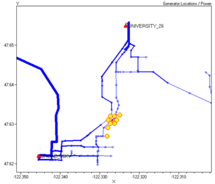
Note: You can change the relative size of the daisy plot circles.
Set daisysize=2 ! Makes the daisy circles twice as large
Set daisysize=0.5 ! Makes the daisy circuit half as large.
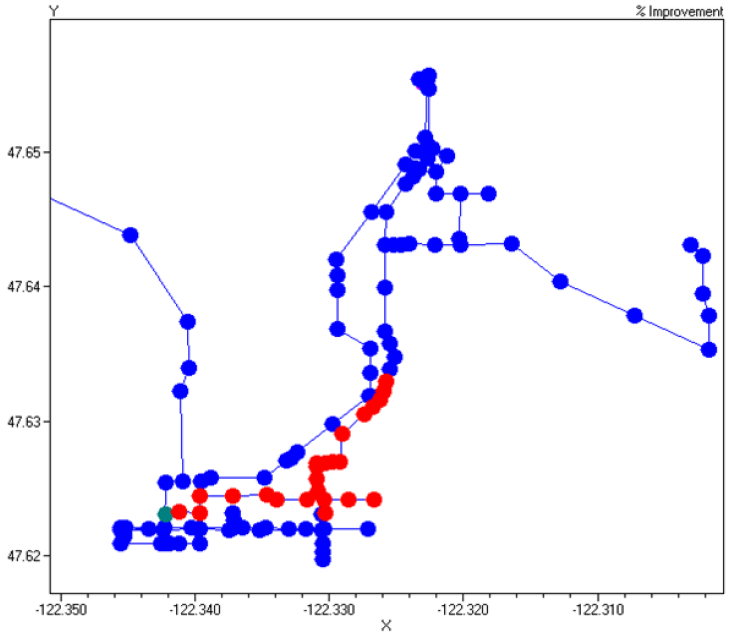
AutoAdd Plot:
This plot displays values from the AutoAddLog.CSV file for the most recent autoadd solution. In this case, the improvement in losses is indicated by color of the nodes. The red nodes have the highest (top 10%, typically) improvement (reduction); the green nodes are next and the blue nodes have the least improvement. This gives some idea where the next optimal position will be.
Results
At the conclusion of the process, the AutoAddedGenerators.txt file will contain DSS script definitions of the generators that were added so that the final results can be duplicated. The improvement factor is noted as a comment in the script. As more generators are added, the improvement declines. The expression “(1, 1)” indicates the relative weighting on losses and capacity, respectively. You will typically look for the clusters in the daisy plot and consolidate the definitions into larger sizes. For example, if you had a 1 MW generator to add, the best location would be near bus “load_lb210”.
New, generator.Gadd1, bus1="load_lb210", phases=3, kv=26.4, kw=100, 1.00! Factor = 0.000612428763446946 (1, 1)
New, generator.Gadd2, bus1="load_lb210", phases=3, kv=26.4, kw=100, 1.00! Factor = 0.000624852211911868 (1, 1)
New, generator.Gadd3, bus1="load_lb210", phases=3, kv=26.4, kw=100, 1.00! Factor = 0.000619740946500293 (1, 1)
New, generator.Gadd4, bus1="load_lb210", phases=3, kv=26.4, kw=100, 1.00! Factor = 0.000610489976851794 (1, 1)
New, generator.Gadd5, bus1="load_lb210", phases=3, kv=26.4, kw=100, 1.00! Factor = 0.000601031100949507 (1, 1)
New, generator.Gadd6, bus1="load_lb1492", phases=3, kv=26.4, kw=100, 1.00! Factor = 0.00059226797914258 (1, 1)
New, generator.Gadd7, bus1="load_lb210", phases=3, kv=26.4, kw=100, 1.00! Factor = 0.000583389649912265 (1, 1)
New, generator.Gadd8, bus1="2604_9", phases=3, kv=26.4, kw=100, 1.00! Factor = 0.000575083882767684 (1, 1)
New, generator.Gadd9, bus1="lb210", phases=3, kv=26.4, kw=100, 1.00! Factor = 0.000566741110334608 (1, 1)
New, generator.Gadd10, bus1="2604_10", phases=3, kv=26.4, kw=100, 1.00! Factor = 0.000558881697352129 (1, 1)