(VSCCS) Voltage-Controlled-Current-Source
This is a power conversion element that interfaces a nonlinear time domain model, in the Hammerstein-Wiener (HW) framework, to the OpenDSS dynamics mode. The model senses terminal voltage and updates the injected current at each OpenDSS time step. Figure 1 shows the relationship between HW and OpenDSS domains, and it defines the key signal locations to reference when reading the Delphi code. In a snapshot mode, the model injected current will be constant, as determined by its ratings and initial power output level. The initial application is for photovoltaic (PV) inverter modeling, and the parameters are defined in those terms. The PV inverter models began with a project sponsored by EPRI at the University of Pittsburgh [1], and they are intended to fill a gap between very detailed [2] and very simple [3] models. The models have since been updated with a phase-locked loop (PLL) implementation for use in protection studies [4]1.
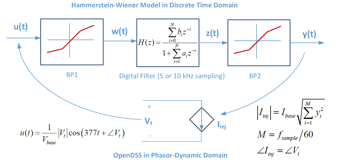
Figure 1: Interface between HW and OpenDSS solution variables
VCCS Input Parameters
Input parameters are listed below. The HW components in Figure 1 work on per-unit variables, so the user may only need to adjust Ppct, Prated and Vrated for specific applications. There are now two available VCCS operating modes, flagged by the value of RMSmode.
• Basefreq: as other PC elements (assumed 60 in Figure 1)
• BP1: XYCurve defining the input piecewise linear block in Figure 1; not used in RMS mode.
• BP2: XYCurve defining the output piecewise linear block in Figure 1; not used in RMS mode.
• Bus1: as other PC elements
• Enabled: as other PC elements
• Filter: XYCurve defining the infinite impulse response (IIR) digital filter coefficients in Figure 1. X values are the numerator coefficients and Y values are the denominator coefficients, and note that a0=1 must be input explicitly. This also enforces equal order in numerator and denominator. In RMSmode, this is typically a second-order digital filter implementation of the phase-locked loop, but other control dynamics in a fast-phasor model could be implemented in this H(z).
• Fsample: sampling rate for H(z), either 5 kHz or 10 kHz in this project. The time step should be an integer multiple of the sample step.
• Imaxpu: for RMSmode only, the nominal maximum current injection in per-unit of rated current.
• Irmstau: for RMSmode only, the time constant of a low-pass filter injecting RMS current from the controller.
• Like: as other PC elements
• Phases: as other PC elements, but only 1-phase implemented now. 3-phase under development.
• Ppct: real power output in snapshot mode, based on Prated. Unity power factor assumed.
• Prated: inverter’s rated power in Watts
• Spectrum: as other PC elements, but not implemented here.
• Vrated: rated line-to-line voltage (3-phase) or line-to-neutral voltage (1-phase) in volts
• Vrmstau: for RMSmode only, the time constant of a low-pass filter sensing RMS voltage.
HWPLL.DSS and HWPLL3.DSS
This file illustrates a second-order phase-locked-loop (PLL) controller in phasor domain . The H(z) defined in lines 5-7 implements a second-order PLL with some overshoot, seen in the blue trace of Figure 2 (left). This overshoot is not actually injected into the circuit because of the 50 ms irmstau time constant specified in line 10, with effect seen in the magenta trace. Based on the sensed rms voltage, i.e., the black trace, the VCCS calculates Ipwr (red trace) to maintain the pre-event real power output. However, Ipwr is affected by H(z) and then Irmstau. Figure 2 (right) shows the per-unit voltage and current at the VCCS terminals. In this example, H(z) and the time constants have been chosen to provide clear illustration of their impacts; these are not necessarily typical values for a real inverter.
Clear
new circuit.HWPLL
~ basekv=4.16 pu=1.0 angle=0 phases=3 bus1=SourceBus
~ r1=0.029 x1=0.058 r0=0.014 x0=0.029
New XYcurve.z_pll npts=3
~ xarray=[ 1.0000 -1.9852 0.9853] // denominator
~ yarray=[ 0.0000 0.0148 -0.0147] // numerator
New vccs.pv Phases=1 Bus1=SourceBus.1 Prated=125e3 Vrated=2400 Ppct=100
~ filter='z_pll' fsample=10000 rmsmode=true imaxpu=1.15
~ vrmstau=0.01 irmstau=0.05
new fault.flt bus1=Sourcebus.1 phases=1 r=0.001 temporary=yes ontime=0.1
new monitor.invvi element=vccs.pv terminal=1 mode=0
new monitor.invst element=vccs.pv terminal=1 mode=3
Set Voltagebases=[4.16]
set maxiterations=100
calcv
set mode=snap
solve
set mode=dynamic
set stepsize=0.0001 // 0.0001 matches fsample
set number=2500 // 2500 matches fsample
Solve
plot type=monitor obj=invvi channels=[1 3] bases=[2400 52.083]
plot type=monitor obj=invst channels=[1 2 3 4]
Figure 3 shows the voltage, current, and power injection from a 3-phase version of this inverter, rated 375 kW at 4160 V line-to-line. The input file is distributed as HWPLL3.dss. The state variable outputs are very similar to Figure 2 (left) for the single-phase inverter. The three-phase inverter continues to produce current and power on the unfaulted phases during the single line to ground fault.
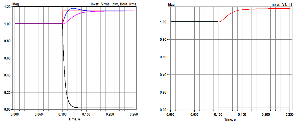
Figure 2: Phasor-mode 1-phase VCCS results for controller state variables (left) and the terminal voltage and current (right).
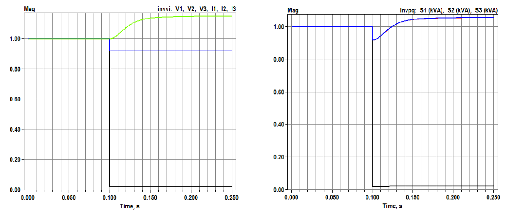
Figure 3: Phase-mode 3-phase VCCS voltages and currents (left) and apparent powers (right).
HWTest.DSS
This file illustrates two inverter models in a snapshot solution. The inverters are connected to a 360-volt source, which matches the lab tests done at 208 volts. The short circuit current supplied by the source is 7354 amps. When phases=3, the VCCS component works in snapshot mode, but not yet in dynamics mode. BP1, BP2, Filter and Fsample have no effect in snapshot mode. The initial currents will be

Clear
new circuit.HWTest
~ basekv=0.360 pu=1.0 angle=0 phases=3 bus1=SourceBus r1=0.02 r0=0.02 x1=0.02 x0=0.02
redirect HW_Inverters.txt
New VCCS.PV1 Phases=1 Bus1=SourceBus.1 Prated=3000 Vrated=208
~ Ppct=100 bp1='bp1_1phase' bp2='bp2_1phase' filter='z_1phase' fsample=10000
New VCCS.PV3 Phases=3 Bus1=SourceBus Prated=3000 Vrated=360
~ Ppct= 50 bp1='bp1_1phase' bp2='bp2_1phase' filter='z_1phase' fsample=10000
Set Voltagebases=[0.360]
set maxiterations=100
calcv
solve
HWDyn.dss
The file that runs a dynamics test has been set up to run either the single-phase inverter or the microinverter, feeding a bolted fault with source impedance adjusted to match that of Pitt’s electric power lab. The fault’s ontime value will determine when the HW model departs from its initial condition. In this case, Fsample is 10 kHz, so the OpenDSS time step must be at least 0.1 ms, but it can be longer. The HW model can run at a faster time step within each OpenDSS time step.
Clear
// EPSL impedance is 10% on 75 kVA positive sequence, 5% zero sequence, assume X/R = 2
new circuit.HWDynamic
~ basekv=0.360 pu=1.0 angle=0 phases=3 bus1=SourceBus r1=0.029 x1=0.058 r0=0.014 x0=0.029
redirect HW_Inverters.txt
New vccs.pv Phases=1 Bus1=SourceBus.1 Prated=3000 Vrated=208 Ppct=100
~ bp1='bp1_1phase' bp2='bp2_1phase' filter='z_1phase' fsample=10000
//New vccs.pv Phases=1 Bus1=SourceBus.1 Prated=190 Vrated=208 Ppct=89.5
//~ bp1='bp1_micro' bp2='bp2_micro' filter='z_micro' fsample=10000
new fault.flt bus1=Sourcebus.1 phases=1 r=0.001 temporary=yes ontime=0.1
new monitor.invvi element=vccs.pv terminal=1 mode=0
new monitor.invpq element=vccs.pv terminal=1 mode=1
new monitor.invst element=vccs.pv terminal=1 mode=3
new monitor.fltvi element=fault.flt terminal=1 mode=0
Set Voltagebases=[0.360]
set maxiterations=100
calcv
set mode=snap
solve
set mode=dynamic
set stepsize=0.01 // 0.0001 matches fsample
set number=25 // 2500 matches fsample
solve
HW_Inverters.txt
This included file defines BP1, BP2, and a 14th-order filter for the microinverter, listed below. The single-phase inverter data is formatted the same way, but it has a 51-order filter, which means its transient response will last longer.
// library model for microinverter
New XYcurve.bp1_micro npts=3
~ xarray=[-0.882023 0.0 0.882023]
~ yarray=[-0.19 0.0 0.19]
New XYcurve.bp2_micro npts=5
~ xarray=[-0.085467 -0.0202 0.0 0.0202 0.085467]
~ yarray=[ 4.59572 1.0 0.0 -1.0 -4.59572]
New XYcurve.z_micro npts=14
~ xarray=[ 1.0000000000000 -1.3802100241988 -0.9341004900495 1.1196620891546 0.1499829369937 1.2123723040884 -0.7654392492287 -0.9113338678997 0.3694835076144 0.1034830928158 0.1549604084080 -0.2209879303901 0.1373924816843 -0.0352249177928 ] // denominator
~ yarray=[ 0.0000000000000 -0.2328126380366 0.9436331671129 -0.5290906112039 -1.2586072419992 0.6136072759695 0.5705618604200 1.0000000000000 -0.5053547399078 -1.1387058093285 -0.0677012182563 0.5067831545610 0.4003099336092 -0.3026288423351 ] // numerator
Example BP1 and BP2
Sample non-linear blocks for the single-phase inverter are shown in Figure 4. They do not necessarily display appropriate symmetry and offset characteristics. Work is ongoing to improve the stability of the fitted model, some of which has been reflected in the non-linear blocks defined in HW_Inverters.txt listed previously. Note that BP2 decreases with X, which required a bug fix to the XYCurve object in OpenDSS for reverse lookup. It’s possible that InvControl is also affected by this fix.
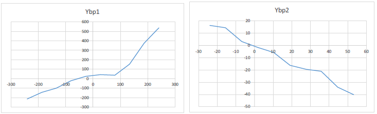
Figure 4: Sample 10-point nonlinear blocks BP1 and BP2
Single-phase Inverter Sample Outputs
Figure 5 shows the single-phase inverter model running at OpenDSS time steps of 0.1 ms. On the left, internal HW model current waveform is in black, RMS in red and peak in blue. The model initialization is smooth, but steady state is not well established until about 0.1 seconds elapse. The red trace on the left is the per-unit RMS current injected into the feeder network. On the right, this is plotted in Amps.
In Figure 5, the OpenDSS time step matches the HW model time step. When OpenDSS runs at a slower time step, the HW model still runs internally at Fsample=10 kHz. However, the output is only sampled at the slower time step, and the current injections are only updated at the slower time step. Figure 6 shows this effect. Especially at 10 ms time step, the waveform is “choppy” but the RMS vs. time is not affected very much.
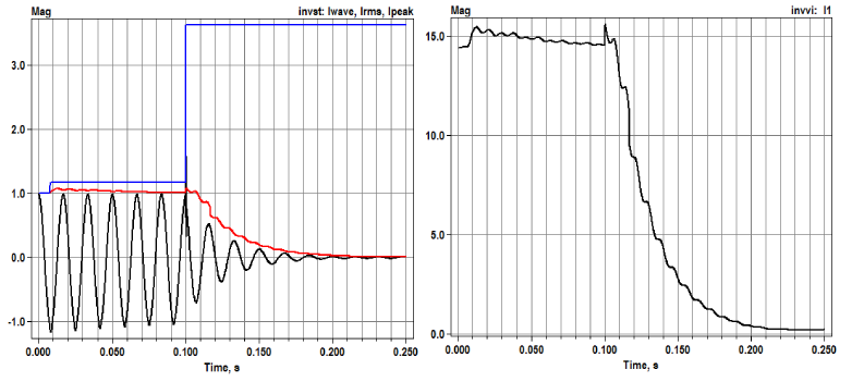
Figure 5: Current waveform, RMS and peak state variables [per-unit] for single-phase inverter. h=0.1 ms (left) and injected
current into the feeder [Amps] (right)

Figure 6: Current waveform, RMS and peak state variables [pu] for single-phase inverter. h=1 ms (left) and 10 ms (right)
Microinverter Sample Outputs
Figure 7 shows a microinverter response to the same fault. With a 14th-order filter at 10 kHz sampling rate, the transient response is shorter in duration. Initialization is smooth, but the accuracy could be improved. The model captures a transient current peak that loads the inverter terminal voltage. When OpenDSS runs at a step longer than 0.1 ms, this loading effect is not captured because the RMS function Pacific Northwest National Laboratory smooths the current peak. Therefore, the peak current is reduced when the OpenDSS time step increases, shown in Figure 6 compared to Figure 5, or Figure 8 compared to Figure 7.

Figure 7: Microinverter current state variables [per-unit] (left) and injected current into the feeder [Amps] (right) at h=0.1 ms.
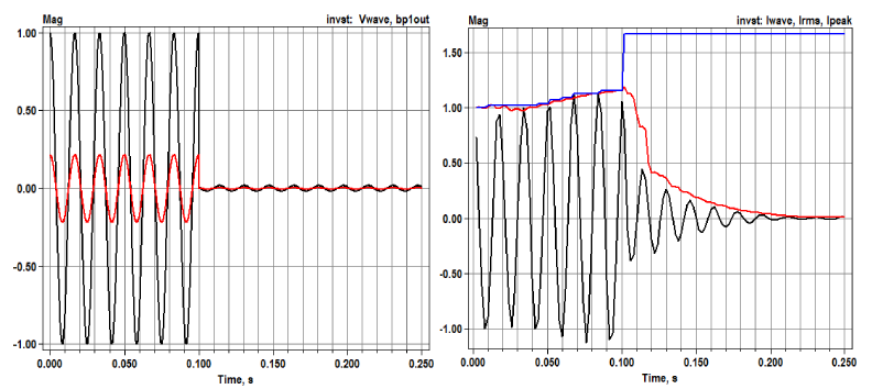
Figure 8: Microinverter voltage state variables (left) and current state variables (right) at h=2 ms.
Code Listings
The most significant parts of the VCCS code define, initialize, and integrate the state variables. Listings follow.
Evaluating H(z) in Figure 1 requires history storage for both input and output. A second copy of both history terms is required for the predictor and corrector steps. Otherwise, when the OpenDSS and HW steps are unequal, the last step’s history could be corrupted by a partial update before the corrector step initiates. The history terms are z, whist, zlast and wlast, allocated to a size determined from the base and sampling frequencies. A ring buffer indexing scheme is used to manage this storage, with helper functions MapIdx and OffsetIdx.
The overloaded InitStateVars procedure extracts terminal voltage and current from the most recent snapshot solution. Then it steps back in time at the sampling frequency to initialize the history terms. The history of z is determined from the history of current, i, passed in reverse through BP2. The HW model current uses generator convention while the OpenDSS current uses passive convention, leading to a negative sign on the initial values of z.
The overloaded IntegrateStates procedure is called twice in each OpenDSS time step, first as predictor (Forward Euler) and then as corrector (Backward Trapezoidal). Each time, it extracts terminal voltage and ensures that whist and z begin afresh from the previous OpenDSS time step. Then, it runs through the BP1, z, and BP2 evaluations defined in Figure 1 for the number of sampling steps contained in an OpenDSS time step. RMS current is calculated “brute force” at the end of the OpenDSS time step, for both predictor and corrector. This value, sIrms, is later injected into the grid via the overloaded procedure GetInjCurrent (not listed below). Note that the current angle updates are not yet implemented. The peak current state variable is checked every HW step to catch “fast” peaks that might not appear in monitor output. The other state variables, and the wlast / zlast history terms, are only updated at each OpenDSS corrector time step.
private
Fbp1: TXYcurveObj;
Fbp1_name: String;
Fbp2: TXYcurveObj;
Fbp2_name: String;
Ffilter: TXYcurveObj;
Ffilter_name: String;
BaseCurr: double; // line current at Ppct
BaseVolt: double; // line-to-neutral voltage at Vrated
FsampleFreq: double; // discretization frequency for Z filter
Fwinlen: integer;
Ffiltlen: integer;
Irated: double; // line current at full output
Fkv: double; // scale voltage to HW pu input
Fki: double; // scale HW pu output to current
// Support for Dynamics Mode - PU of BaseVolt and BaseCurr
sVwave: double;
sIwave: double;
sIrms: double;
sIpeak: double;
sBP1out: double;
sFilterout: double;
vlast: complex;
y2: pDoubleArray;
z: pDoubleArray; // current digital filter history terms
whist: pDoubleArray;
zlast: pDoubleArray; // update only after the corrector step
wlast: pDoubleArray;
sIdxU: integer; // ring buffer index for z and whist
sIdxY: integer; // ring buffer index for y2 (rms current)
y2sum: double;
// helper functions for ring buffer indexing, 1..len
function MapIdx(idx, len: integer):integer;
begin
while idx <= 0 do idx := idx + len;
Result := idx mod (len + 1);
if Result = 0 then Result := 1;
end;
function OffsetIdx(idx, offset, len: integer):integer;
begin
Result := MapIdx(idx+offset, len);
end;
// support for DYNAMICMODE
// NB: The test data and HW model used source convention (I and V in phase)
// However, OpenDSS uses the load convention
procedure TVCCSObj.InitStateVars;
var
d, wt, wd, val, iang, vang: double;
i, k: integer;
begin
// initialize outputs from the terminal conditions
ComputeIterminal;
iang := cang(Iterminal^[1]);
vang := cang(Vterminal^[1]);
sVwave := cabs(Vterminal^[1]) / BaseVolt;
sIrms := cabs(Iterminal^[1]) / BaseCurr;
sIwave := sIrms;
sIpeak := sIrms;
sBP1out := 0;
sFilterout := 0;
vlast := cdivreal (Vterminal^[1], BaseVolt);
// initialize the history terms for HW model source convention
d := 1 / FsampleFreq;
wd := 2 * Pi * ActiveSolutionObj.Frequency * d;
for i := 1 to Ffiltlen do begin
wt := vang - wd * (Ffiltlen - i);
whist[i] := 0;
whist[i] := Fbp1.GetYValue(sVwave * cos(wt));
wlast[i] := whist[i];
end;
for i := 1 to Fwinlen do begin
wt := iang - wd * (Fwinlen - i);
val := sIrms * cos(wt); // current by passive sign convention
y2[i] := val * val;
k := i - Fwinlen + Ffiltlen;
if k > 0 then begin
z[k] := -Fbp2.GetXvalue (val); // HW history with generator convention
zlast[k] := z[k];
end;
end;
// initialize the ring buffer indices; these increment by 1 before actual use
sIdxU := 0;
sIdxY := 0;
end;
// this is called twice per dynamic time step; predictor then corrector
procedure TVCCSObj.IntegrateStates;
var
t, h, d, f, w, wt: double;
vre, vim, vin, scale, y: double;
nstep, i, k, corrector: integer;
vnow: complex;
iu, iy: integer; // local copies of sIdxU and sIdxY for predictor
begin
if not Closed[1] then begin
ShutoffInjections;
exit;
end;
ComputeIterminal;
t := ActiveSolutionObj.DynaVars.t;
h := ActiveSolutionObj.DynaVars.h;
f := ActiveSolutionObj.Frequency;
corrector := ActiveSolutionObj.DynaVars.IterationFlag;
d := 1 / FSampleFreq;
nstep := trunc (1e-6 + h/d);
w := 2 * Pi * f;
vnow := cdivreal (Vterminal^[1], BaseVolt);
vin := 0;
y := 0;
iu := sIdxU;
iy := sIdxY;
for k := 1 to FFiltlen do begin
z[k] := zlast[k];
whist[k] := wlast[k];
end;
for i:=1 to nstep do begin
iu := OffsetIdx (iu, 1, Ffiltlen);
// push input voltage waveform through the first PWL block
scale := 1.0 * i / nstep;
vre := vlast.re + (vnow.re - vlast.re) * scale;
vim := vlast.im + (vnow.im - vlast.im) * scale;
wt := w * (t - h + i * d);
vin := (vre * cos(wt) + vim * sin(wt));
whist[iu] := Fbp1.GetYValue(vin);
// apply the filter and second PWL block
z[iu] := 0;
for k := 1 to Ffiltlen do begin
z[iu] := z[iu] + Ffilter.Yvalue_pt[k] * whist[MapIdx(iu-k+1,Ffiltlen)];
end;
for k := 2 to Ffiltlen do begin
z[iu] := z[iu] - Ffilter.Xvalue_pt[k] * z[MapIdx(iu-k+1,Ffiltlen)];
end;
y := Fbp2.GetYValue(z[iu]);
// updating outputs
if (corrector = 1) and (abs(y) > sIpeak) then
sIpeak := abs(y); // catching the fastest peaks
// update the RMS
iy := OffsetIdx (iy, 1, Fwinlen);
y2[iy] := y * y; // brute-force RMS update
if i = nstep then begin
y2sum := 0.0;
for k := 1 to Fwinlen do y2sum := y2sum + y2[k];
sIrms := sqrt(2.0 * y2sum / Fwinlen); // TODO - this is the magnitude, what about angle?
end;end;
if corrector = 1 then begin
sIdxU := iu;
sIdxY := iy;
vlast := vnow;
sVwave := vin;
sBP1out := whist[sIdxU];
sFilterout := z[sIdxU];
sIwave := y;
for k := 1 to FFiltlen do begin
zlast[k] := z[k];
wlast[k] := whist[k];
end;
end;
end;
DG_Prot_Fdr.dss
Our last example illustrates use of the VCCS model in an IEEE test feeder for DG protection analysis. See Figure 9, with feeder data defined in [5]. The DG was originally assumed to contribute fault current as a rotating machine, but here the source is a PV inverter, represented with a VCCS. Note that the VCCS does not emulate solar panel efficiency, power fluctuations, or smart inverter control; for those features, please use other components of OpenDSS (e.g. PVSystem, InvControl, ExpControl). In Figure 9, we will apply single-line-to-ground faults (SLGF) at the feeder mid-point location, bus Bm or fault location 3.

Figure 9: IEEE test feeder for DG protection analysis [5]
Here is a partial listing of the test file DG_Prot_Fdr.dss, showing the 1.7 MVA wind turbine generator commented out, and an equivalent 1.7 MW PV generator comprised of single-phase inverters. In either case, a 1700-kVA wye/wye interconnection transformer interfaces the DG to the primary feeder.
// DG interconnection transformer and a conventional machine
new Transformer.Tg phases=3 windings=2 buses=(Bt Bg) conns=(Wye Wye)
~ kvs='12.47 0.36' kvas='1700 1700' taps='1 1' XHL=5
//new Vsource.WindGen1 bus1=Bg basekv=0.36 pu=1.0 angle=-48.5
//~ X1=0.0127 R1=0.0 X0=100.0 R0=0.0
redirect HW_Inverters.dat
New vccs.pv1 Phases=1 Bus1=Bg.1 Prated=567e3 Vrated=208 Ppct=100
~ bp1='bp1_1phase' bp2='bp2_1phase' filter='z_1phase' fsample=10000
New vccs.pv2 Phases=1 Bus1=Bg.2 like=pv1
New vccs.pv3 Phases=1 Bus1=Bg.3 like=pv1
// Inverter Model Monitors
new monitor.invst1 element=vccs.pv1 terminal=1 mode=3
new monitor.invst2 element=vccs.pv2 terminal=1 mode=3
new monitor.invst3 element=vccs.pv3 terminal=1 mode=3
new monitor.invvi element=vccs.pv1 terminal=1 mode=0
new monitor.invpq element=vccs.pv1 terminal=1 mode=1
Figure 10 shows the current and voltage through recloser B, on the high side of the interconnection transformer, with a 1700-kW PV inverter source back-feeding the fault at Bm. The fault occurs at 0.2 seconds, just after steady-state DG output currents have stabilized. The faulted phase voltage (Figure 10 right) collapses almost immediately. Figure 11 shows the same fault response for a Thevenin equivalent source in place of the PV. The Thevenin impedance is sized to produce 6 pu short-circuit current at the source terminals based on 1700 kVA. The initial power is 1721 kW. As a result, the fault contribution is higher and the feeder primary voltage on the faulted phase, at recloser B, is maintained at a low level indefinitely.

Figure 10: Per-unit currents (left) and voltages (right) at recloser B with 1.7 MW PV and single-phase inverter models
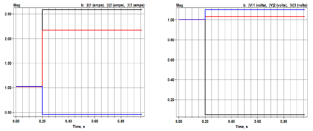
Figure 11: Per-unit currents (left) and voltages (right) at recloser B with 1.7 MW rotating machine (Thevenin equivalent)
The same case can be run with a three-phase PLL model of the inverter. In the next segment of DG_Prot_Fdr.dss, a voltage relay has been added to shut off the inverter when the undervoltage or overvoltage trip levels from IEEE 1547-2008 have been exceeded. In rmsmode, the VCCS injects only positive-sequence current, which contributes to stability of the simulation.
New XYcurve.z_pll npts=3
~ xarray=[ 1.0000 -1.9852 0.9853] // denominator
~ yarray=[ 0.0000 0.0148 -0.0147] // numerator
New vccs.pv Phases=3 Bus1=Bg Prated=1700e3 Vrated=360 Ppct=100
~ filter='z_pll' fsample=10000 rmsmode=true imaxpu=1.15
~ vrmstau=0.01 irmstau=0.05
new Relay.LV monitoredobj=vccs.pv type=voltage kvbase=0.36 switchedobj=vccs.pv
~ overvoltcurve=ov1547 undervoltcurve=uv1547 shots=1 delay=0.0
Results are shown in Figure 12 and Figure 13. During the first 0.2 seconds, the PLL reduces the current to produce rated power at the 1.07 per-unit pre-fault terminal voltage. After the fault, the PV inverter contributes up to 1.15 per-unit current on each phase through the interconnection transformer.

Figure 12: DG protection feeder fault with PLL model, p.u. state variables (left), recloser B p.u. voltages and currents (right).

Figure 13: DG protection feeder fault with PLL model, p.u. inverter sequence currents (left), and voltages (right).
The faulted positive sequence voltage drops to about 0.7 per-unit, so the inverter injects 1.15 positive sequence current during the fault, both shown in Figure 13. However, the inverter shuts down at about 0.36 seconds because Relay.LV tripped on low voltage. As Figure 12 (right) indicates, the faulted phase voltage drops below 0.1 per-unit during the fault. Because of the wye-wye transformer connection, Relay.LV sees this voltage directly and trips 0.16 seconds after the fault.
References
[1] L. M. Wieserman, "Developing a Transient Photovoltaic Inverter Model in OpenDSS Using the Hammerstein-Wiener Mathematical Structure," PhD, Electrical and Computer Engineering, University of Pittsburgh, Pittsburgh, 2016. [Online]. Available: http://d-scholarship.pitt.edu/30339/1/wiesermanlm_etdPitt2016.pdf
[2] M. E. Ropp and S. Gonzalez, "Development of a MATLAB/Simulink Model of a Single-Phase Grid-Connected Photovoltaic System," IEEE Transactions on Energy Conversion, vol. 24, no. 1, pp. 195-202, 2009, doi: 10.1109/TEC.2008.2003206.
[3] L. Wieserman and T. E. McDermott, "Fault current and overvoltage calculations for inverter-based generation using symmetrical components," in 2014 IEEE Energy Conversion Congress and Exposition (ECCE), 14-18 Sept. 2014 2014, pp. 2619-2624, doi: 10.1109/ECCE.2014.6953752.
[4] L. M. Wieserman, S. F. Graziani, T. E. McDermott, R. C. Dugan, and Z. Mao, "Test-Based Modeling of Photovoltaic Inverter Impact on Distribution Systems," in 2019 IEEE 46th Photovoltaic Specialists Conference (PVSC), 16-21 June 2019 2019, pp. 2977-2983, doi: 10.1109/PVSC40753.2019.8980968.
[5] T. E. McDermott, "A test feeder for DG protection analysis," in Power Systems Conference and Exposition (PSCE), 2011 IEEE/PES, 20-23 March 2011 2011, pp. 1-7, doi: 10.1109/PSCE.2011.5772608.
1 This material is based upon work supported by the U.S. Department of Energy’s Office of Energy Efficiency and Renewable Energy (EERE) under Solar Energy Technologies Office (SETO) Agreement Number 34233.