Calculation of the smart inverter function
In this section is to calculate the desired reactive power, qDfun[t]j, and/or the active power limit, pLfun[t]j, according to the modes below:
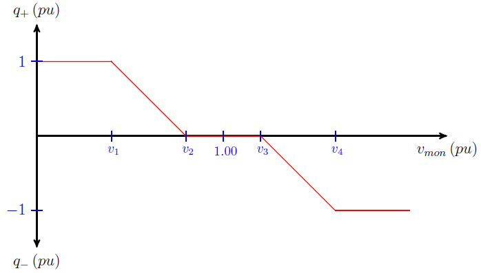
Smart Inverter volt-var Function For the smart inverter volt-var function, the monitored voltage in pu is applied , vmon[t]j, in the volt-var curve defined in the vvc_curve1 property to obtain the desired reactive power value in pu, qDfun[t]j. The Figure 9 below shows an example of an user-defined volt-var curve.
The desired reactive power in pu can be written according to Equation 53.

Smart inverter DRC function For the smart inverter DRC function, the desired reactive power value is set according to Equation 54.

Where the voltage difference is calculated according to Equation 55.

And vwindowdrc [t]j corresponds to the mean of the voltages of the averaging window of the DRC function. This average voltage is calculated according to Equation 56 considering that the averaging window can store the voltages of m previous time steps. The time-scale length of this window is set in the DynReacavgwindowlen property.
Combined Smart inverter volt-var and DRC function For the combined mode of the smart volt-var and DRC functions, the desired reactive power value is the sum of the result of Equation 53 and Equation 54, according to Equation 57.

Smart inverter volt-watt function For the smart inverter volt-watt function, the monitored voltage in pu is applied, vmon[t]j, in the volt-watt curve defined in the voltwatt_curve property to obtain the active power limit value in pu, pLfun[t]j. The Figure 10 shows an example of a user-defined volt-watt curve.
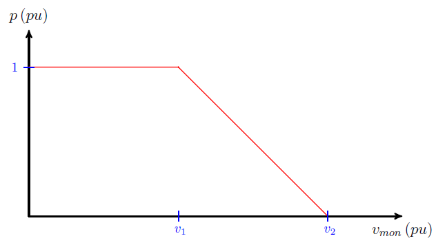
The active power limit value in pu is calculated as shown in the Equation 58.

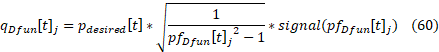
Smart inverter watt-pf function For the smart inverter watt-pf function, the output active power in pu is applied, pdesired[t], in the watt-pf curve defined in the wattpf_curve property to obtain the power factor, Equation 59, and then calculate the desired reactive power value in pu, qDfun[t]j, according to Equation 60. The Figure 11 shows an example of an user-defined watt-pf curve.

One can notice that the watt-pf curve, Figure 11, has the nominal/reference point in power factor 1 instead of 0. As a result, the user needs to define this watt-pf curve based on a curve that has its reference in power factor equal to 0, according the Figure 12. The discontinuity in p2 is not a problem due to the reactive power is zero for either power factor equal 1 or -1.
To define this watt-pf curve, the user needs to calculate the p2, and include the coordinates (p2, 1) and (p2, -1) into the OpenDSS XYcurve object.
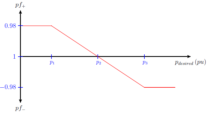
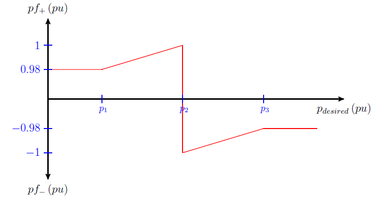
Figure 12: watt-pf curve with reference in zero
Smart inverter watt-var function For the smart inverter watt-var function, the output active power in pu is applied, pdesired[t], in the watt-var curve defined in the wattvar_curve property to obtain the desired reactive power value in pu, qDfun[t]j, according to Equation 61. The Figure 13 shows an example of a user-defined watt-var curve.
