Constant PF Mode
To illustrate the storage operation in the constant PF mode, the Follow active power self-dispatch mode has been considered. The script used is similar to the one in previous examples apart from the
differences in the dispatch curve and the addition of storage element property pf = −0.90.
New LoadShape.dispatch_shape interval=1 npts=24
~ mult=[0.0,0.01,0.08,0.12,0.16,0.30,0.50,0.88,0.0,0.0,0.0,0.0,0.0,0.0,0.0,0.01,0.08,0.12,0.16,0.30,0.50,0.88,0.0,0.0]
New Storage.Storage1 phases=3 bus1=A kv=0.48 pf=1 kWrated=50 %reserve=20
~ effcurve=Eff kWhrated=500 %stored=50 state=idling
~ dispmode=follow pf=0.90 model=1 daily=dispatch_shape
Figure 13 shows the active and reactive powers at the interface with the grid. Note that because of the negative power factor, the reactive power has an opposite sign to the active power. Figure 14 shows the PQ plane with the resulting operating points throughout the simulation. All points are over the constant -0.9 power factor line, even during idling state.
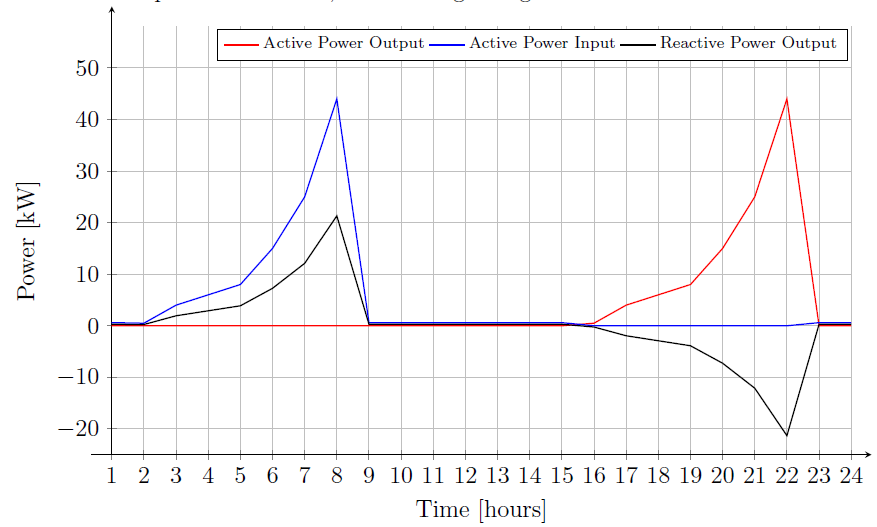
Figure 13. Powers at Storage Interface
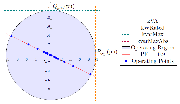
Figure 14. PQ Plane with Inverter Capability Curve and Operating Points under Constant PF Mode