Norton equivalent
This section presents the Norton equivalent definition for a three-phase PVSystem connected to the grid through the bus named as Connection Bus, as presented in Figure 7.
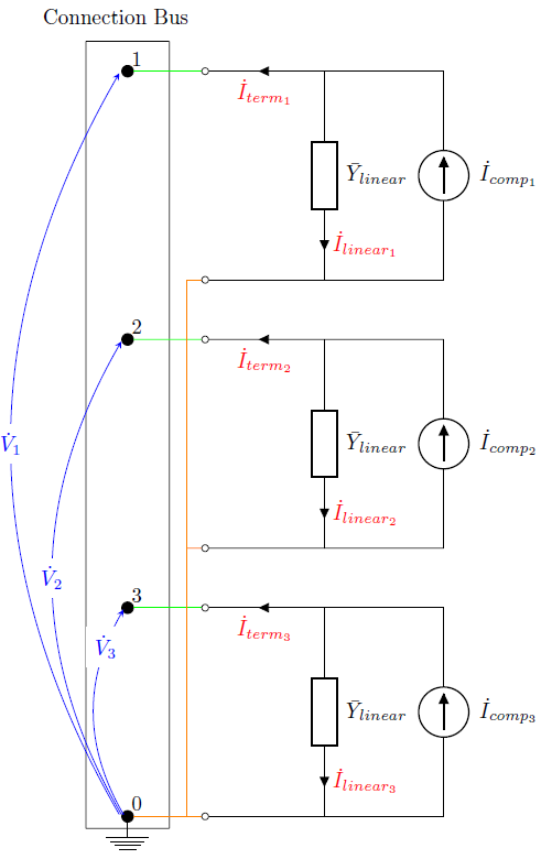
Figure 7: A three-phase PVSystem modeled as a Norton Equivalent
By observing Figure 7, the following electric quantities can be defined:
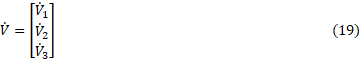
- Nodal voltages:
˙ ˙
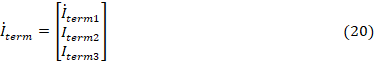
- Terminal currents:
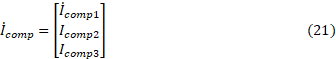
- Norton or compensation currents:
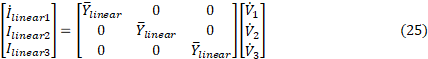
- Linear currents:

The normal power flow solution technique in OpenDSS is based on the Equation 23.

Where:
- I˙: Injected current array;
- V˙ : System voltage array.
OpenDSS computes the compensation currents from each PC element to populate the injected current array. Therefore, the main purpose of this section is to understand how OpenDSS calculates the compensation currents for PVSystem. It means: I˙comp1 , I˙comp2 and I˙comp3
It is possible by means of Kirchhoff’s first law to express the compensation currents in function of the linear and terminal currents, as presented in Equation 24.

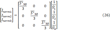
The linear currents can be written as a function of the nodal voltages, Equation 25, and the terminal currents as a function of both the three-phase apparent power provided by the PVSystem , S¯3φ, and the nodal voltages, Equation 26. (It is assumed that PVSystem operates with constant power).
The Norton or linear admittance, Y¯linear , is calculated using the apparent power provided by the element, according to Equation 27.

Where:
- Vn corresponds the rated voltage of the PVSystem.
The final expression for the calculation of the compensation currents, therefore, is presented in Equation 28.

The compensation currents are calculated as shown above if two conditions are satisfied. First, the model property of the PVSystem is set equal to 1, the default OpenDSS value for constant power operation. And second, each nodal voltage has to be in the range defined by the Vminpu and Vmaxpu properties, which by default are 0.9 and 1.1, respectively. Outside this range, the corresponding phase of the element is modeled as constant impedance.