OpenDSS Documentation

In this example, the storage controller is set to operate in peakshave mode for discharging and time mode for charging. The peakshaving target is 10MW with the default band of +/-1%. The charging is set to start at 2am, with a rate of 50%. The power monitored by the controller in peakshave mode is at the first terminal of the same line where a monitor has been placed in the base script and the fleet reserve has been set to 20%.

Edit Storage.F kWrated=100 

Edit Storage.G kWrated=125

/*

s e t  casename=NoEnergy

Edit Storage .A kWhrated=250 % stored=70 

Edit Storage . B kWhrated=500 % stored=70 

Edit Storage . C kWhrated=825 % stored=70

Edit Storage .D kWhrated=625 % stored=70 

Edit Storage . E kWhrated=250 % stored=70 

Edit Storage . F kWhrated=600 % stored=70 

Edit  Storage .G kWhrated=625  % stored=70

*/

! S o l uti o n  S e t t i n g s

Set maxcontroliter=50 

Set mode=Daily

Setstepsize=1h

Set number=24

Solve

Export monitors m1pq

Export Eventlog

Export monitors storage.Astates

Export monitors storage.Bstates

Export monitors storage.Cstates 

Export monitors storage.Dstates 

Export monitors storage.Estates

Export monitors storage.Fstates

Export monitors storage.Gstates

Three different cases are run. In the first one, named “Complete”, no changes are applied to the fleet ratings, which is enough to completely shave the peak, as shown in Figure 9. In the second one, “NoPower”, the rated power of each element of the fleet is reduced in 50%. In this case, it can be seen that the fleet is not able to totally shave the peak from 6pm to 8pm. In the last case, the total energy capacity of the fleet has been reduced to 50% of its original value. Because of that, the fleet reaches its reserve energy at 9pm, and cannot continue to shave the peak after that.

Note that the total necessary time to charge the fleet at the beginning of the day is different for each case due to different power and energy rated capacities. Also note the little increase in the power measured when the fleet is idling, due to the existence of idling losses.

Figure 10 shows the power dispatched by each element of the fleet for the complete shaving case. At the beginning of the day, indeed, each element charges with 50% of their respective rated power. In time mode, as explained in section 5.3.2, the fleet remain in the state set by the controller until there is no longer enough capacity left in the fleet, which can occur at different time instants for each element depending on each element’s ratings. For instance, element E takes only three hours to be fully charged, while element F takes 5 hours. This can also be seen in Figure 11.

Table 2 shows the event log with all control actions executed by the controller. Note that the controller sets the fleet to discharge the first time at 6pm, when the regulated power is greater

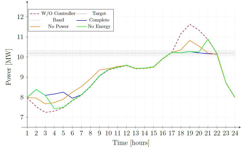
Figure 9: Powers at the monitored line element for each PeakShaving case

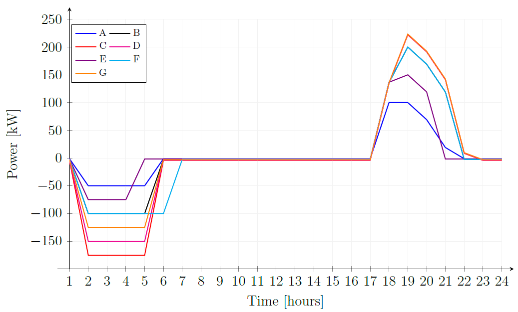
Figure 10: Power output at each element of the fleet for the case with complete shaving

than the specified target band for the first time (see the power monitored in the case without any storage elements and controller in the circuit). The power requested by the controller to element A is limited to its rated power (Equation 2). All other elements are requested the same power increment. Take elements B and F , for instance. The total power needed to drive the regulated power to the target is 969.34kW . As the fleet is constituted by 7 elements and they are all given the same weight (see Weights property), the incremental change of power requested is 138.48kW . As their power consumption during idling state is 2kW (1% of kWRated) due to idling losses plus 0.43kW due to the corresponding inverter losses (taken from the data exported from monitors storage B states and storage F states), the power requested to these two elements is 138.48 − 2.43 = 136.05kW .

As the system’s loading increases to the peak, at 7pm, the controller requests more power from elements B to G. The amount of incremental power requested is enough to reach storage’s E, F and B rated power, 150kW , 200kW and 200kW , respectively. The other three remaining elements’ rated power is enough to fulfill the requested power necessary to fully shave the peak. See in Table 2 that it requires an extra control iteration to accomplish this.

At 8pm, the system’s loading starts to decrease. Thus, the controller requests the fleet to reduce its dispatch. Note that because the controller operates by requesting incremental changes in the power dispatched, the entire fleet gets its dispatched power reduced by the same amount: 215.108 = 30.73kW .

At 9pm, storage E is completely depleted, as shown in Figure 11. Thus, the controller does not send any dispatch request to this element. However, the decrement in the power requested to the other six elements is enough to drive the regulated power to the band around the 10.2 MW target. Then, the controller does not push any other actions to the control queue in the second control iteration.

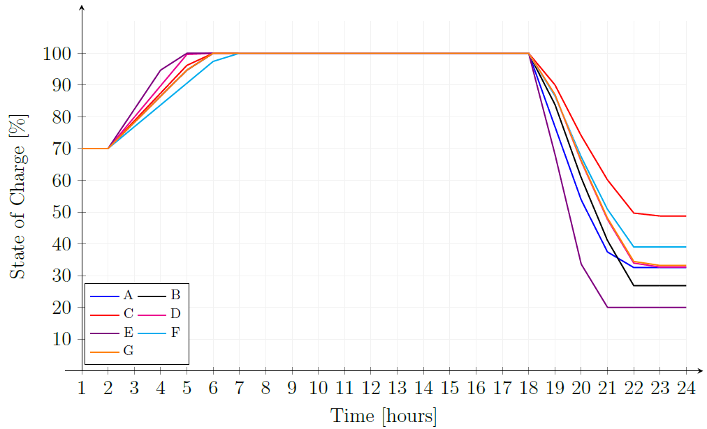
Figure 11: State of charge of each element of the fleet for the case with complete shaving

At 10pm, the total loading reduction leads the controller to decrement the total requested power in 778.753kW , which means that each element is requested to reduce its dispatch by more than 110kW in the first control iteration. However, as storage E is already idling, only the other 6 elements receive the request. As storage A is dispatching less than 50kW at 9pm, the resulting power would be negative, so the element goes into idling state.

The resulting reduction (lower than the required) in the regulated power from the power flow of the next control iteration is not enough to drive it to the target value. Thus, the controller sends new actions (dispatch requests) in the second control iteration. In this iteration, the necessary power

dispatch reduction is only 149.9kW. The power change requested to the fleet also leads storages B

and F to go into idling state.

In the third control iteration, the power flow is solved again and the regulated power is finally within the target band. Thus, no more control action are required. Then, at 10pm only storages C, D and G remain in discharge mode and are responsible for shaving the peak.

Finally, at 11pm the system’s loading reduces significantly and the controller sets these three element to idling state as well.

Table 2: Event log of PeakShaving in the simulation case with complete shaving

1. Effect of MonPhase property

In the previous example, as the property MonPhase has been set to AV G. This means that the regulated measure used by the controller is the total three-phase power of the monitored line at the specified terminal, which is, in fact, the power shown in Figure 9. However, as shown in Figure 12,

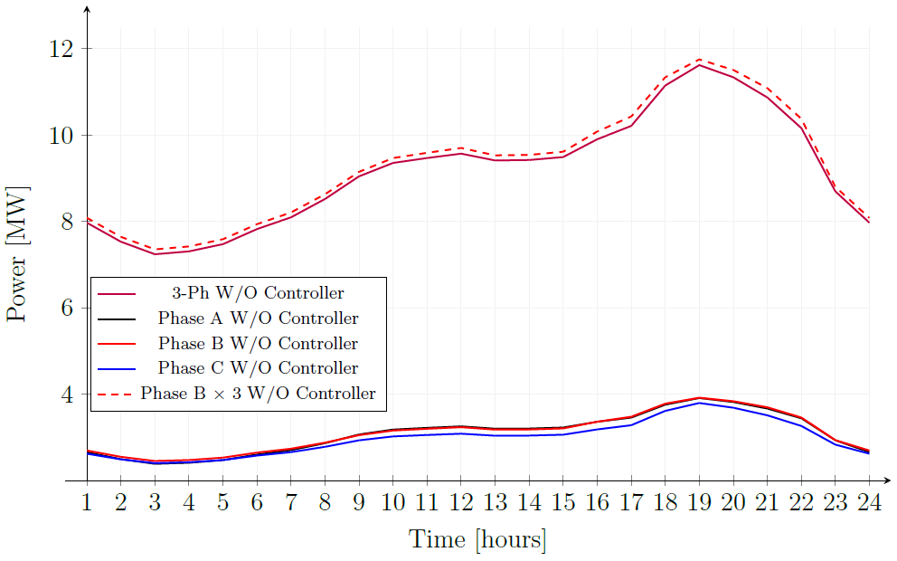
Figure 12: Powers at the monitored element without controller

the simulated circuit is unbalanced. In this case, MonPhase may be useful. It allows the user to select a measure in a specific phase to be the controller input value. Consider that we would like to shave the peak adopting the most loaded phase, which is phase B (nodes “2” in the MV level, MonPhase = 2). As the monitored element is a 3-phase line, the controller will assume the actual power at the specific location is 3 times the measured quantity, shown in Figures 12 and 13.

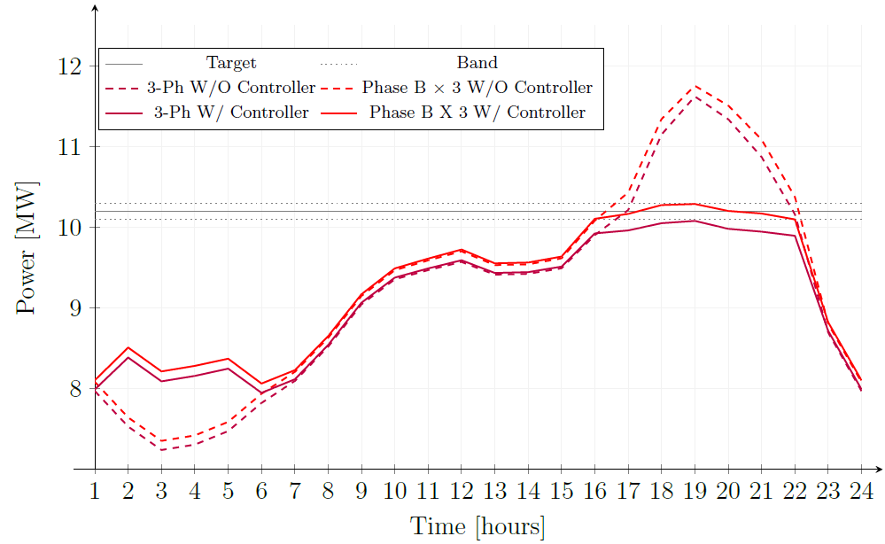
Figure 13: Powers at the monitored element for PeakShaving with MonPhase = 2

Figure 13 shows that, indeed, the controller regulates the monitored value to the target band. The practical effect is that the actual three-phase power measured stays below the specified target. This would be useful if there is a meter monitoring only a single phase. Supposing that the loading of each phase varies throughout the day such that one phase is the most loaded one during a specific period but not for others, the user could also use MonPhase = MAX instead (which is the default value), and the controller would look for the most loaded phase at every single time step.

The intent of this property is to guarantee that the controller would not let the power in any individual phase to be overloaded. Note that if MonPhase = AV G, the regulation of the total 3-phase active power does not mean that the single-phase power in each phase is within the acceptable range if there is significant unbalance.