Default Mode
In the script presented below, a loadshape is first created to be used as the dispatch curve to drive the storage operation. Since the simulation is performed in daily mode, in the storage definition, it is assigned to the Storage element daily property. Note that the element’s initial state is set to idling and its initial SOC is set to 50%. Figure 6 presents the evolution of the element SOC, dispatch curve, and charging and discharging triggers. Figure 7 shows the element input and output active powers, and the storage inverter, idling, charging/discharging, and total losses. The curves have been plotted from the data exported from a monitor attached to the storage in mode 3.
!StorageOperationinDefaultDispatchMode\
Clear
New Circuit.Source bus1=A basekv=0.48 phases=3pu=1
New LoadShape.dispatch_shape interval=1 npts=24
~ mult=[0.380,0.220,0.247,0.280,0.313,0.370,0.589,0.672,0.7477,0.832,
0.88,0.94,0.989,0.985,0.98,0.9898,0.999,1.0,0.958,0.936,0.913,
0.800,0.720,0.610]
!Inverter Efficiency Curve
New XYCurve.Eff npts=4 xarray=[.1 .2 .4 1.0] yarray=[.86 .9 .93 .97]
New Storage.Storage1 phases=3 bus1=A kv=0.48 pf=1 kWrated=50 %reserve=20
~ effcurve=Eff kWhrated=500 %stored=50 %idling kW=2 state=idling
~ dispmode=default model=1 daily=dispatch_shape
~ chargeTrigger=0.34 dischargeTrigger=0.85
New Monitor.MonStorage1State element=Storage.Storage1 mode=3
New Monitor.MonStorage1Powers element=Storage.Storage1 mode=1 ppolar=No
Set voltagebases=[0.48]
Calcvoltagebases
Set mode=Daily
Solve
Plot Monitor object=MonStorage1State channels=(123478910)
Plot Monitor object=MonStorage1Powers channels=(135)
The storage element operation is discussed below in detail for the different time periods:
- 1am - 2am : The storage SOC is 50% (250 kWh) and the storage is operating in idling state (initial state) absorbing the power necessary to supply its idling losses and associated inverter losses. No state change is requested as the dispatch curve is greater than ChargeTrigger and less than DischargeTrigger;
- 2am - 6am : At 2am, the dispatch curve becomes less than ChargeTrigger, so the storage changes to charging mode charging at the rated power, kWRated;
- 6am - 11am : At 6am, the charging is ceased as the dispatch curve exceeds the ChargeTrigger;
- 11am - 5pm : At 11am, the storage starts to discharge at rated power, kWRated, as the dispatch curve exceeds the DischargeTrigger. At 5pm, the discharging is suspended as the stored energy reaches its reserve level (100 kW, 20% of kWhRated) even though the dispatch curve stays above DischargeTrigger;
- 5pm - 12am : The element stays in idling state;

Figure 6. Stored Energy, Dispatch Curve and Triggers
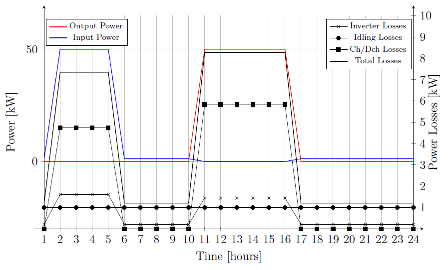
Figure 7. Powers at Storage Interface and Power Losses
Note that the storage total losses 2-6am are different to the storage total losses 11am-5pm even though the power at the storage grid interface is equal between these two periods (but with different directions). This fact is in agreement with the storage element internal power flow discussed in sections 5.1 and 5.2. In charging state, the power at the input of the charging losses block is equal to the power at the grid interface, 50 kW, minus the inverter and idling losses, whereas in discharging state, the power at the input of the discharging losses block is the sum of the output power, the inverter and idling losses and the discharging losses itself, according to equations 2 and 7, respectively. The inverter losses also differ between charging and discharging states but less than the charging/discharging losses.
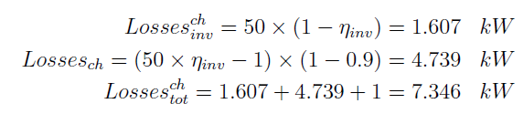
As ηch e ηdisch have not been specified, both are equal to their default value 90%. The idling losses are 2% of the rated power, which is equal to 1kW. Consider two time instants: one with the storage charging and second with the storage discharging. Following the equations shown in section 5, the storage losses during these two time instants can be described as shown below.
In charging state, the inverter efficiency (based on the inverter efficiency curve) for 50kW power at the grid interface is ηinv ∼= 0.968 (extracted from the report exported from monitor in mode 3). The losses are given by:
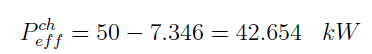
Thus, the power that effectively charges the storage is
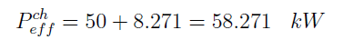
In discharging state, the inverter efficiency curve (based on the inverter efficiency curve) for 50kW power at the grid interface is ηinv ∼= 0.972 (extracted from the report exported from monitor in mode 3). The losses are given by:

Thus, the power that effectively discharges the element is
We encourage the user to run the script of this example and to export the state variables from monitor “Mon Storage1 State” to verify these results.