Price and LoadLevel Modes
As these modes are very similar, the storage operation is illustrated only for the Price mode. In the script below, a PriceShape object has been defined as an hypothetical energy price that varies throughout the day. Note that the definition of this object is very similar to a LoadShape object. The PriceShape element is assigned to the global price curve, pricecurve. Figures 10 and 11 show the resulting storage operation.
!Storage Operation in Price Mode
Clear
New Circuit.Source bus1=A basekv=0.48 phases=3 pu=1
New PriceShape.Price interval=1 npts=24
~ price=[75,68,67,69,71,75,75,80,80,80,90,90,90,95,95,95,105,105,110,110,110,90,90,90]
!Inverter Efficiency Curve
New XYCurve.Eff npts=4 xarray=[.1 .2 .4 1.0] yarray=[.86 .9 .93 .97]
New Storage.Storage1 phases=3 bus1=A kv=0.48 pf=1kWrated=50 %reserve=20
~ kWhrated=500 %stored=50 state=idling debugtrace=yes dispmode=price model=1
~ dischargeTrigger=100 chargeTrigger=74
New Monitor.MonStorage1State element=Storage.Storage1 mode=3
New Monitor.MonStorage1Powers element=Storage.Storage1 mode=1 ppolar=No
Set voltagebases=[0.48]
Calcvoltagebases
Set pricecurve=Price
Set mode=Daily
Solve
Plot Monitor object=MonStorage1State channels=(1234567)
Plot Monitor object=MonStorage1Powers channels=(135)
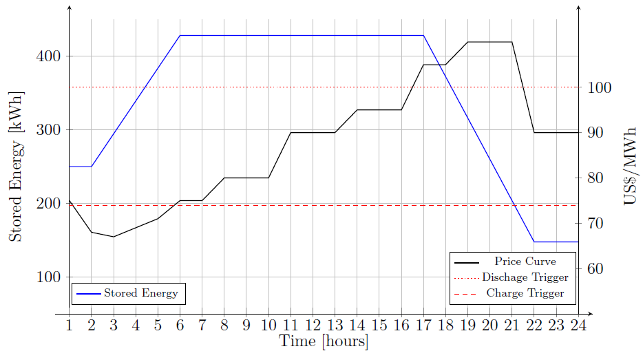
Figure 10. Stored Energy, Price Curve and Triggers.
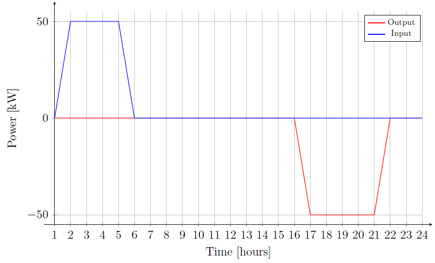
Figure 11. Powers at Storage Interface