Reactive Power Violation
This example illustrates the violation of reactive power limit in several violation regions. It also shows a different inverter capability curve shape from the previous ones.
....
!Reactive Power Violation(linear region,kvar Max,kVA)
New LoadShape.dispatchFollow interval=(13600/) npts=24 mult=[0,0.01,0.08,0.12,0.14,0.16,0.30,0.50,0.6,0.8,0.95,0,0.01,0.08,0.12,0.14,0.16,0.30,0.50,0.6,0.8,0.95,0,0]
Edit Storage.Adisp mode=follow daily=dispatchFollow %cutin=0 %cutout=0
~ %PminNoVars=0 kvarMaxAbs=600 %idlingkW=0
!VVCurve
New XYCurve.vvcurve npts=5 yarray=[1 1 0 1 1] xarray=[0.5 0.92 1.0 1.08 1.5]
New InvControl.InvCtrl combiMode=VVDRC dbVMin=1 dbVMax=1 arGraLowV=50
~ arGraHiV=50 dynReacAvgWindowLen=2 srefReactivePower=VARMAX vvccurve1=vvcurve
~ varChangeTolerance=0.001
!PPriority
Set casename=Ppriority
Edit Storage.Awattpriority=true
!QPriority
!Setcasename=Qpriority
!EditStorage.Awattpriority=false
Set mode=Daily
Set maxcontroliter=50
Set stepsize=1s
!13am
Edit VSource.source pu=1.0
Set number=3
Solve
!4am
Edit VSource.source pu=0.98
Set number=1
Solve
!5am
Edit VSource.source pu=0.96
Solve
!6am
Edit VSource.source pu=0.94
Solve
!7am
Edit VSource.source pu=0.92
Solve
!8am
Edit VSource.source pu=1.05
Solve
!910am
Edit VSource.source pu=1.00
Set number=2
Solve
!11am
Edit VSource.source pu=0.97
Set number=1
Solve
!12pm3pm
Edit VSource.source pu=1.00
Set number=4
Solve
!4pm
Edit VSource.source pu=1.03
Set number=1
Solve
!5pm
Edit VSource.source pu=1.06
Solve
!6pm
Edit VSource.source pu=1.1
Solve
!79pm
Edit VSource.source pu=0.98
set number=3
Solve
!10pm
Edit VSource.source pu=1.16
set number=1
Solve
!11pm12am
Edit VSource.source pu=1.0
Set number=2
Solve
Export monitors MonStorageAState
Export monitorsMonStorageAV
Export eventlog
Similarly, to the previous example, the storage element is operated with active power driven by “Follow” mode. The properties %CutIn, %CutOut, %PminNoVars and %idlingkW have been set to 0 and kvarMaxAbs has been set to 600 kvar to modify the shape of the inverter capability curve.
The reactive power dispatch is driven by an InvControl control element, through VV and DRC smart inverter functions, which have been enabled through property combimode. For more details about the other InvControl properties used, see [2]. As in this reactive power dispatch mode constant PF priority is not applicable, the simulation is run considering active and reactive power priorities only. The time step size has been set to 1 second, which is more appropriate for the DRC function.
As in the previous examples, the magnitude of the voltage source is varied throughout the simulation to force the InvControl to request different reactive power levels to the storage element. In this case, the voltage has been intentionally varied such that the inverter operates in all four quadrants throughout the simulation. Figure 9 shows the PQ plane with all operating points for both priorities.
Note that the reactive power reaches several boundaries: kV A, kvarMax, kvarMaxAbs and the boundaries in the region of ascending linear reactive power limit (in quadrants II and IV). Besides that, note that the operating point differs between the two priorities considered for some operating points in which they apparently should be the same (highlighted in Figure 9). There are two reasons for that. The first one is due to the nature of the DRC function, which considers a moving average (with a time window of 2 seconds in this example) of the voltage at the element’s terminal to calculate the requested reactive power. The second is that there is a difference between the moving average calculated at some time instants only because they happen right after a time instant in which there has been a kVA violation. Thus, the different priorities set different final complex power operating points, and, as a consequence, different voltages, leading to different reactive power requests by the DRC function in the following time steps. As the moving average acts as low-pass filter, the response for the two different priorities eventually converge to the same value after a few later time steps. The user is encouraged to run the examples and verify this fact.
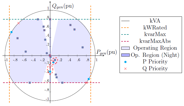
Figure 9: PQ Plane with Inverter Capability Curve and Operating Points for Operation Driven by an InvControl in VV+DRC